STRUCTURES Blog | The Beauty of Gaussian Random Fields

How do scientists describe and predict complex patterns and structures emerging in nature, signals or data? Is there a straightforward method to reduce the complexity even of systems as big and complex as the entire universe itself, without losing information we might be interested in? Remarkably, several such methods exist and are frequently used by physicists and mathematicians. Today we want to look at one particularly simple, yet powerful method: Gaussian Random Fields. Gaussian Random Fields are ubiquitious and provide a statistical tool for describing a vast amount of different structures all over nature, from electronics to geography, and from machine learning to cosmic structures.

Gaussian Random Fields are an example for a statistical description of data. A statistical description provides a simple summary of a data sample, by representing it in terms of a small number of macroscopic quantities that capture the information of interest. What makes Gaussian Random Fields special is that they require very simple assumptions and only two parameters to understand the key properties of many structures encountered in nature. This is because in numerous situations, the properties of such structures arise from stochastic processes with independent random variables. Random fields are functions taking random values at different points in a parameter space. A random field is Gaussian if these numbers are drawn from a Gaussian probability distribution.

Reminder: Gaussian normal distribution

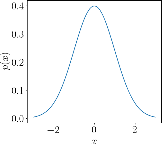
The Gaussian distribution is a continuous probability distribution that is symmetric about its mean and describes data that is more frequent near the mean than far away. In $d$ dimensions, the (multivariate) Gaussian probability density function $p(\mathbf x)$ is given by

$$ p(\mathbf{x}) = \frac{1}{\sqrt{(2\pi)^d \lvert\Sigma\rvert}} \exp{ \left( -\frac{1}{2}(\mathbf{x} - \mathbf{\mu})^T \Sigma^{-1} (\mathbf{x} - \mathbf{\mu}) \right)}, $$

where $\mathbf x$ is the vector of input variables (data), $\mu$ is the mean and $|\Sigma|$ is the determinant of the covariance matrix $\Sigma$.

The special case for one dimension ($d = 1$) is shown in the plot on the left. For the standard normal distribution the mean is zero and the value of the standard deviation is one. It has zero skew and a kurtosis of three. In graphical form, the normal distribution appears as a "bell curve". Many naturally-occurring phenomena tend to approximate the normal distribution.

Gaussian Random Fields are ubiquitious. They are a natural consequence of many processes due to the law of large numbers, and hence very common to observe. From a theoretician’s point of view, treating a random field as Gaussian simplifies mathematical considerations vastly. In the following, we want to focus on a particular simple case: homogeneous and isotropic Gaussian Random Fields. Here, we will encounter what is known as white noise and we will understand why it is called like that.

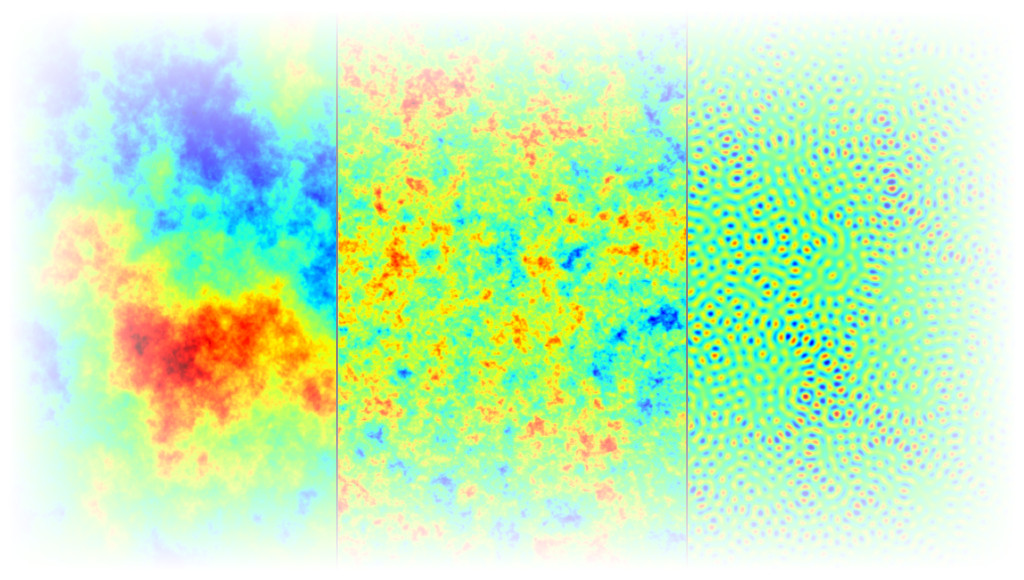
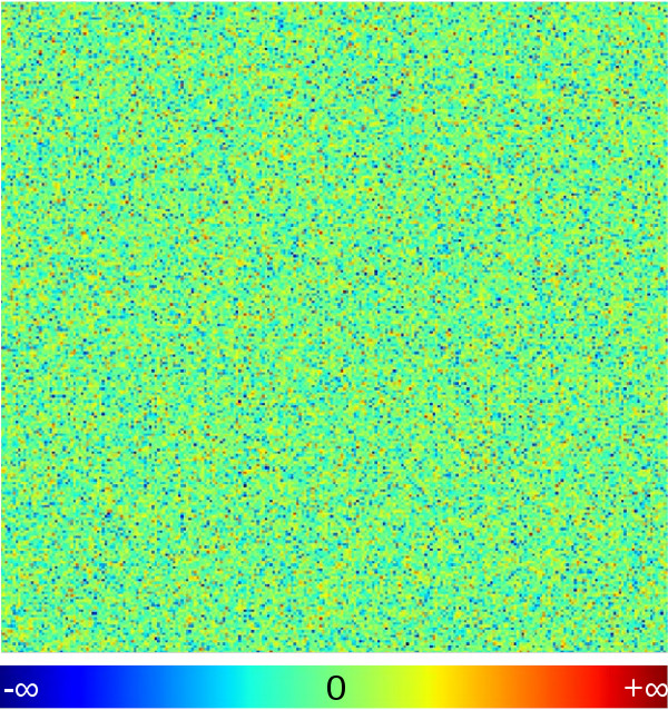
For simplicity, we restrict our discussion to two-dimensional Gaussian Random Fields on a discrete grid. You can picture the “field” in this case as an infinitely extended “pixelised image”. Now what about the randomness? We want to assign a (random) number to each pixel. This way, we initialise our random field. We draw these numbers from a Gaussian distribution to arrive at a Gaussian random field. An example showing the result of such a procedure is visualised in Fig. 1, where the colours correspond to different field values. Given that all pixels are assigned independent random numbers, there is no structure in this image. We then say the image is free of correlations. That is, when knowing the colour of one pixel, without looking at the image, we cannot guess anything about the colour of a neighboring pixel – except that it was drawn from the same Gaussian distribution.

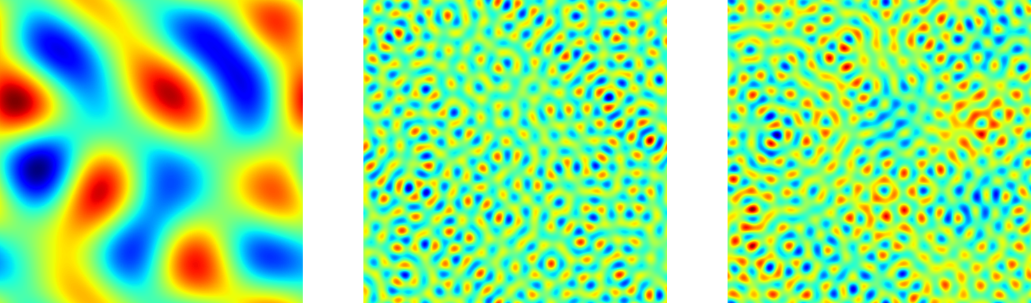
This is an image with 256 x 256 pixels. For each pixel, a random number was drawn from a Gaussian centered around a mean of 0, and with a variance of 1. To visualise the result, the numbers were mapped to a colour bar.

How does a Gaussian Random Field look when there are correlations? Let’s consider the exact opposite of the scenario we studied in Fig. 1, i.e. a scenario in which we have as much correlation as possible. This means we want to create a field in which knowing the colour of one pixel immediately lets you guess the colour of all other pixels correctly: the pixels shall be perfectly correlated. This can be achieved if all the pixels have equal colors, e.g. by drawing a single random number from a Gaussian and assigning this number to all pixels in the field. Three instances of such a maximally correlated field are shown in Fig. 2. They correspond to different realisations of the maximally correlated Gaussian random field.

The three images show three independent instances of a perfectly correlated Gaussian random field with 256 x 256 pixels each. Since the pixels in each individual image are perfectly correlated, all pixels have the same colour. Colour bar is the same as in Fig. 1.

Blobby patterns and the correlation function

So what happens if we introduce just a little amount of correlation? We saw that the absence of any correlation creates unstructured noise, whereas perfect correlations lead to perfectly structured plain images. Correlations provide a measure of deviation from randomness. No correlations means that the color of one pixel contains no information about the color of another pixel. What if we want a field with structures, where for example nearby pixels have similar colours? First, we have to specify what we mean by “nearby”. This is where the concept of correlation length comes into play. The correlation length defines an average length scale on which pixels are correlated with each other. In addition, we need to specify “how” similar the colours should be. This corresponds to the “strength” or “amplitude” of correlations. We can also demand that pixels separated by some distance should have colours as different as possible. In this case, we speak of “anti-correlated” field values at a certain distance.

Formally, correlations are the distance-dependent second cumulant of the random field. For simplicity, we will assume that our field has no dependence on direction (i.e. it is isotropic) and looks statistically the same everywhere when large enough scales are considered (i.e. it is homogeneous). This is, for instance, the case for cosmic matter density fluctuations in the early universe, which at least at early times define an isotropic and homogeneous Gaussian random field. In such a case, the correlations can depend only on the distance between pixels. In order to compute the corresponding correlation function, which specifies the amplitude of correlation for given distances, it turns out we simply need to multiply the field values $f_1, f_2$ of two pixels at a given distance $\Delta x $ and average the result over all pixel pairs with this distance.

In the case of uncorrelated pixels, this will yield as many pixel pairs with opposite sign as with equal sign. Thus, the average over all these numbers is zero. If pixels are statistically similar, however, there are more pixel pairs for which the sign of the product is equal than opposite. This gives rise to a positive correlation. For dissimilar pixels, it is exactly the other way around, hence a negative or anti-correlation.

$C (\Delta x) = \langle f(y) \cdot f(y + \Delta x) \rangle_y$

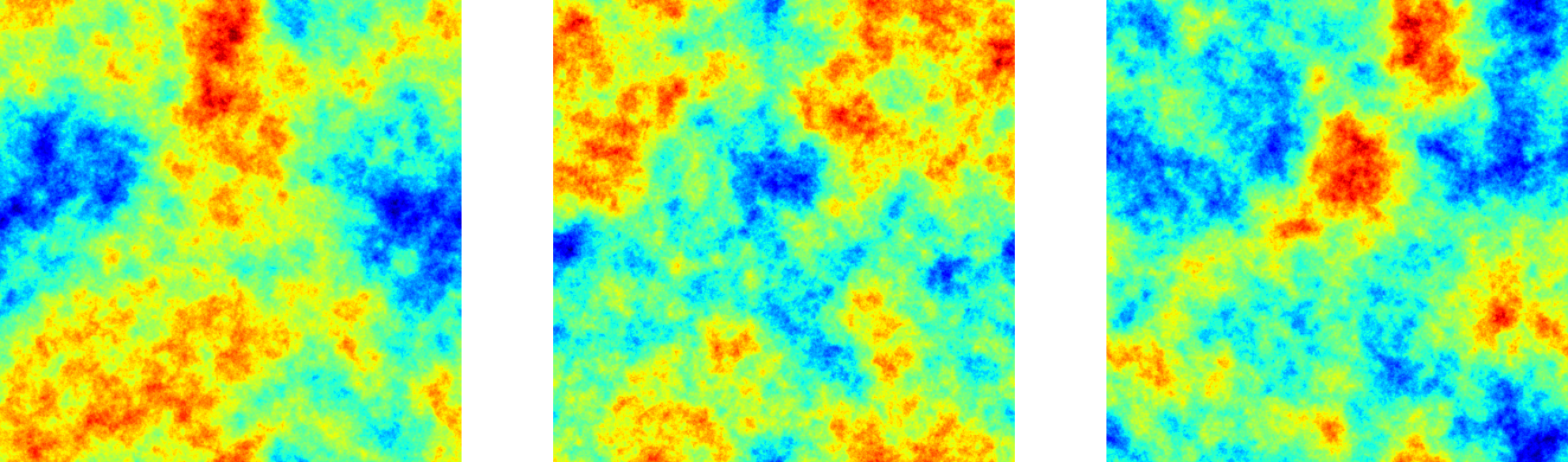
A very nice aspect of Gaussian Random Fields is that the (generally position-dependent) mean pixel value and the correlation function (giving the second cumulant) describes the statistics of the random field completely. Fig. 3 shows how blob patterns of various blob sizes can be generated when the correlation function is an oscillating cosine: nearby pixel values and pixels separated by an even multiple of the correlation length “$l$” are correlated, while pixels separated by an odd multiple are anti-correlated. Larger blobs correspond to a larger correlation length. In principle, we can also create a pattern of small blobs embedded in larger blobs by simply adding the two correlation functions!

$C(\Delta x) = \cos ( 2 \pi \Delta x / l )$. Left: instanciation of a Gaussian random field with large correlation length. Middle: small correlation length. Left: the total correlation function is the sum of the correlation functions of the left and middle image. Colour bar is the same as in Figure 1.

The power of the power spectrum

Although the correlation function contains all information about correlations in a Gaussian random field, scientists came up with a related measure that more directly quantifies the “size” of structures that typically occur in the field: the power spectrum, which is the Fourier transform of the correlation function:

$P(k) = \int C(x) \mathrm{e}^{ikx} \mathrm d x$

This enables to change from the spatial domain to a frequency domain, as expressed by the argument $k$ of the function, which is the wave number with unit 1/length. For each wave number $k$, the power spectrum indicates the strength of spatial variations in field values at the length scale corresponding to $k$. Coming back to the examples in Fig. 3 with the cosine-shaped correlation functions, the power spectrum strongly peaks at the respective value $k = 1/l$ in the fist two cases and peaks twice at both “$1/l$” in the third case, indicating that $l$ is the typical size of the structures present.

Already without doing any calculation, we can infer the power spectrum expression for the maximally correlated fields we introduced in Fig. 2: given that the field values are equal everywhere up to a separation that extends to infinity, “structures” in these images have an infinite length. Thus, the power spectrum has to peak strongly at a wavelength of $1/l = 0$ and is zero for all non-vanishing values of $k$.

Now we can ask: how do structures look like when the power spectrum is more continuous, i.e. when structures of all sizes are present? A very popular class of Gaussian Random Fields of this category are the so-called scale-free Gaussian Random Fields. These have a power spectrum that falls off like a power law and the structures in these fields are typically fractal. As you may know, power law functions do not distinguish any particular length scale. Thus, no matter how much you zoom in our out, the pattern basically looks the same – ignoring the finite pixel resolution of the grid of course.

$P(k) \propto k^{-\alpha}$. Three instanciations of a scale-free Gaussian random field. The power spectrum is a power law. Therefore, structures of all sizes are present, leading to a fractal structure. But fractals are worth an own, future article ;-). Colour bar is the same as in Figure 1.

Why white noise is called white noise

Coming back to our first Gaussian random field, the uncorrelated picture of Fig. 1, we now focus on the case of so-called white noise, as this scenario is called. Although it might seem unintuitive, the power spectrum of this uncorrelated field is scale free with exponent zero, i.e. flat. You can check this by calculating the Fourier transform of its correlation function, which is a Dirac delta distribution peaking at $Δx = 0$. Thus, the white noise picture is a superposition of blobs of all sizes in a way such that every visible structure is lost! The name white noise directly comes from the resulting shape of the power spectrum: the (auditory) spectrum of acoustic white noise is completely flat, i.e. a superposition of all pitches or frequencies, in a way that no structure in the acoustic signal remains. In our case, we are looking at colours rather than acoustic signals, but the principle is the same: the superposition of electromagnetic waves of all frequencies (and thus of all colours) to equal amount leads to white light. This is why the noisy pattern of Gaussian Random Fields with flat power spectra is called “white”.

Plots are generated using the FyeldGenerator package for python
Licensed under the CC-BY-SA license.