Beautiful Mathematics of Simple Experiments

Mathematicians often face a curious dilemma: while certain concepts are elegantly defined in theory, they can be quite elusive in practice. Take, for example, the definition of π. It is given as the ratio of a circle’s circumference to its diameter. While this definition is exact, it is not very practical for use in a calculator. If we wish to use π in numerical computations, we need approximations, which yield numbers close enough to π that can be computed explicitly, like 3.14159 or ³⁵⁵/₁₁₃.

One classic strategy to approximate π dates back to ancient Greek mathematician Archimedes, who made clever use of geometry. His idea was to approximate a circle with regular polygons from the inside and outside (see Fig. 1a below). As the number of polygon sides increases, these shapes resemble the circle more closely, and their perimeters provide increasingly tight bounds for π. Applying this method for a circle with a diameter of 1 yields the results shown in the table below. On the right-hand side, you can try for yourself: just move the interactive slider below the circle with the polygons to change the number of slides.

Number of Sides	Peri­me­ter of In­scribed Poly­gon	Peri­me­ter of Cir­cum­scribed Poly­gon
4	2.828427	4.000000
16	3.121445	3.182598
64	3.140331	3.144118
256	3.141514	3.141750
1024	3.141588	3.141603

Loading...

But not all approximations play fair. Imagine you had started with a square around the circle and repeatedly “folded” its corners inward to make its shape look more circular (see Fig. 1b). Again, the shape would visually approach a circle, but now something strange happens: its perimeter no longer approaches π. In fact, it no longer changes at all, but remains fixed at a value of 4:

Number of Folds	Peri­me­ter of Shape
0	4
1	4
10	4
100	4
1000	4
10000	4

Loading...

Wait…what just happened? Both algorithms produced shapes that look like circles, but only Archimedes’ polygons correctly approximated π. In the folding case, no matter how many times we folded the corners, the perimeter remained fixed at 4. What we ran into here is an example of a “bad” approximation. But why was it a bad approximation?

Why Some Approximations Lie to You

The answer is that not all notions of “closeness” preserve the features that matter. Just because two shapes look identical, it does not guarantee that their underlying properties – such as perimeter – will behave the same, too. Thus we need to pay careful attention to what stays preserved when things get close.

Mathematicians express the idea of something “getting closer and closer” through various notions of what they call convergence. These offer a rigorous way to talk about how objects – be it numbers, functions, or shapes – approach a specific target (so-called “limit”), which is a fundamental concept encountered throughout mathematics. Importantly, different types of convergence preserve different properties.

When the folded square converges to the circle, it does so in a specific sense: as we fold its corners inward, the area between the folded square and the circle shrinks. This is what mathematicians call L¹-convergence: two shapes get “close” if the area of their mismatch shrinks. But perimeter doesn’t care about area mismatches, it cares about boundary length. Folding the square introduces tiny zigzags that are invisible to L¹-convergence but disastrous for perimeter convergence. In particular, while the zigzags shrink the area mismatch, they don’t shorten the boundary – they merely rearrange it, bringing it closer to the circle. You can see this by observing that all we do when folding a corner is to “cut out” little sections from the outline and shift them horizontally or vertically. As illustrated in Fig. 2, we could simply move all these tiny line segments together to recover the original square. Thus the total length never changes, even though the shape does get arbitrarily close to the circle if we keep folding its corners.

This shows why visual proofs can be deceptive: convergence in one sense may not imply convergence in another. What may look like a good approximation method might not preserve the underlying mathematical properties we’re interested in – in this case the shape’s perimeter.

When Effective Approximation is Key: A Kitchen Experiment

What we just encountered is an example of how some notions of convergence produce better results than others. More generally, whether an approximation is “good” depends on the question you’re asking, and it is the job of the mathematician to determine the right notion of convergence for a given problem.

One very powerful notion of convergence that we encounter in a field called calculus of variations is the concept of “Γ-convergence” (pronounced “gamma convergence”). Introduced by Ennio De Giorgi and Tullio Franzoni in the 1970s, Γ-convergence is a mathematical tool for simplifying certain complex problems while preserving an essential feature: minimization processes. Imagine a situation where you are looking for the most efficient way of achieving something – for instance minimizing cost, time, or energy – but finding this optimal solution, called minimizer, is complicated. Suppose the problem allows us to introduce a “zoom-out parameter” (traditionally called “ε”) that lets us gradually ignore certain fine-scale features. At each zoom level, we’re working with a coarser version of the original problem. Γ-convergence ensures that, as we zoom out, the optimal solutions of our “hard problems” progressively converge towards the optimal solution of the “simple” problem, known as the Γ-limit. Since Γ-convergence ensures that minimizers converge to minimizers, we know that the solution of the simple problem is close to the original, complex problem.

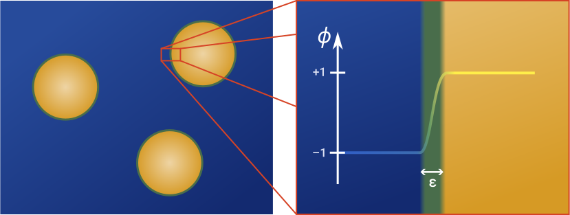
To see Γ-convergence in action, let us perform a classic kitchen experiment: imagine you take a bottle of water and pour a little bit of oil into it. Close the bottle, shake it, and watch: after a short amount of time, the water and oil separate into blobs. Moreover, you will see that the shapes formed by regions of pure water or oil are spherical! Upon a very close look, you will find that the two phases (oil and water) do not split cleanly. Instead, there is a very thin transition layer separating these pure phases of water and oil. In this very thin layer, molecules intermingle in slightly chaotic ways.

In the 1950s, mathematicians John W. Cahn and John E. Hilliard developed a model to capture how materials like oil and water separate into distinct phases. Their model, later extended by Cahn and his collaborator Sam Allen, assigns a notion of energy to the system, which is minimized over time. This energy quantifies the “cost” of the system adopting certain states, for instance mixed or pure regions, or thick or thin transition layers. It turns out that two things are particularly costly: mixed regions of opposite phase and rapid spatial variations in phase. In other words, both too thick or too thin transition layers are costly. These competing factors drive the system to balance both phenomena by forming domains of pure phases (oil or water) separated by a thin but stable transition layer.

For the shape of droplets, physical intuition suggests they should be spherical because of surface tension minimizing their area. However, rigorously proving this requires solving complex equations. Moreover, their predictions depend on a parameter that controls the thickness of the diffuse layer but in real-world systems is vanishingly small – think nanometres for oil-water interfaces – making practical calculations difficult. On the other hand, setting the thickness to zero breaks the model: assuming a model with exactly zero layer thickness would fail to describe realistic phase separation dynamics. In particular, the model would no longer penalize interfaces, so droplets would lose their shape entirely.

Γ-Convergence to the Rescue: From Complexity to Geometric Simplicity

Here is where Γ-convergence comes to the rescue. Instead of solving these complex equations directly, it asks a simple question: What happens to the energy when the transition layer becomes vanishingly thin? In other words, how does it simplify when the interface is almost – but not quite – infinitely sharp? In the 1970-80s, mathematicians Luciano Modica and Stefano Mortola were able to show that in such a “sharp-interface limit”, the Cahn-Hilliard energy Γ-converges to a simple geometric law: to leading order, the energy is proportional to the perimeter of the phase boundary, scaled by a material-dependent constant.

As a result, predicting droplet shapes is no longer about solving complex partial differential equations, but about solving an almost 300-year old geometric problem: finding surfaces with minimal perimeter in a given container. This is now an easy task to solve, as the shapes with minimal perimeter are well-known in this scenario. In particular, these shapes are spheres in the given situation (where the ratio of oil to water is small) – exactly what we see in the corresponding experiment.

Why is it helpful to study the sharp-interface limit? The point of idealizations is not only to make calculations easier (or possible), but to purposefully isolate properties we deem relevant from irrelevant ones. Γ-convergence in this context helps us to bridge scales, allowing us to focus on those properties that become visible in the “greater picture”. For the Cahn-Hilliard example, as we zoom out, the original complex problem with its “messy” microscopic details is replaced by a simple geometric law. This law is entirely independent of material-related properties that did affect the Cahn-Hilliard energy of the original problem. Thus we find that the system displays universal properties emerging in the sharp-interface limit.

For Advanced Readers: Deep Dive Into the Mathematics

You wish to get to know the mathematics? Click here to expand this section!

1. Introducing $\mathrm{\Gamma }$-Convergence

$\mathrm{\Gamma }$-convergence provides a rigorous framework for understanding how a sequence of functionals $F_{\epsilon }$ behaves in the limit $\epsilon \to 0$. Unlike standard notions of convergence (such as pointwise or uniform convergence, which directly compare function values), $\mathrm{\Gamma }$-convergence ensures that, under minimal conditions, minimizers of $F_{\epsilon }$ approximate minimizers of the limiting functional $F_0$. This makes it particularly useful in situations where exact minimization may be too difficult, but one can study an approximate problem in the limit.

Let’s assume we have a sequence of functionals $F_{\epsilon }$ mapping a given system state $x$ to a real number (e.g. a system’s energy). For these functionals we have a corresponding family of minimization problems,

$$F_{\epsilon }[x_{\epsilon }^{\ast }]=min{F}_{\epsilon }[x].$$

Now we ask: for $\epsilon \to 0$, is there a limit functional $F_0$ such that the sequence of minimizers $x_{\epsilon }^{\ast }$ converges to the minimizer $x_0^{\ast }$, i.e. $F_0[x_0^{\ast }]=min{F}_0[x]$?

The answer is yes, $\mathrm{\Gamma }$-convergence provides you with such a limit functional:

Definition: $\mathrm{\Gamma }$-Convergence
A sequence of functionals $F_{\epsilon }:X\to \mathbb{R}\cup \mathrm{\infty }$ defined on a topological space $X$ is said to “$\mathrm{\Gamma }$-converge” to a functional $F_0:X\to \mathbb{R}\cup \mathrm{\infty }$ (the “$\mathrm{\Gamma }$-limit”) if the following two inequalities are satisfied:

1. Liminf Inequality: For every sequence $x_{\epsilon }\in X$ converging to $x\in X$ it holds that:
   $$F_0[x]\le \underset{\epsilon \to 0}{lim inf}{F}_{\epsilon }[x_{\epsilon }].$$ This means $F_0$ is a lower bound for all possible asymptotic behaviours of the sequence $F_{\epsilon }.$
2. Limsup Inequality: For at least one sequence $x_{\epsilon }\in X$ converging to $x$, it holds that:
   $$F_0[x]\ge \underset{\epsilon \to 0}{lim sup}{F}_{\epsilon }[x_{\epsilon }].$$ This states that for at least one asymptotic behaviour of the sequence, $F_0$ provides – at the same time – an upper bound, meaning that the $\mathrm{\Gamma }$-limit is exactly achieved for that sequence. In other words: the lower bound from the liminf inequality is optimal.

The fundamental theorem of $\mathrm{\Gamma }$-convergence then ensures that if $F_{\epsilon }\stackrel{\mathrm{\Gamma }}{⟶}{F}_0$, then minimizers of $F_{\epsilon }$ converge to minimizers of $F_0$.

2. Application to the Cahn-Hilliard Model

As an application example, let us consider the Cahn-Hilliard model, describing the experiment from above. In this model, we study a free energy functional of the form:

$$E_{\epsilon }[\varphi ]=\frac{1}{\epsilon }{\int }_{\Omega }(\frac{{\epsilon }^2}{2}|\mathrm{\nabla }\varphi {|}^2+W(\varphi )\hspace{0.17em})\mathrm{d}V,$$

where $\mathrm{\Omega }\subset {\mathbb{R}}^n$ is a regular bounded region and $\varphi :\mathrm{\Omega }\to \mathbb{R}$ is a phase field that varies smoothly between $-1$ and $+1$ (which describe pure phases, e.g. pure oil or pure water in the oil-water example). The small parameter $\epsilon$ characterizes the thickness of the transition layer between the two pure phases.

The Cahn-Hilliard energy contains two terms whose effects compete against each other:

• The gradient term $|\mathrm{\nabla }\varphi {|}^2$ resists rapid spatial changes in the phase parameter $\varphi$, smoothing the transition layers.

• The term $W(\varphi )$ is a double-well potential that penalizes mixing of phases, favouring separation into distinct “bulk” phases near the minima of $W$. Typical choices include the shapes shown in Fig. 4, and in general depend on details of the materials under consideration.

The framework of $\mathrm{\Gamma }$-convergence rigorously shows that, as $\epsilon \to 0$, the family of functionals $E_{\epsilon }$ $\mathrm{\Gamma }$-converges to the perimeter functional. Digging a little bit deeper, $\mathrm{\Gamma }$-convergence allows for an expansion of the energy (similar to Taylor expansion) in terms of the limiting parameter close to the minimum $\varphi$, i.e.

$${\int }_{\mathrm{\Omega }}({\epsilon }^2|\mathrm{\nabla }\varphi {|}^2+W(\varphi ))\mathrm{d}V=C_W\cdot \epsilon \cdot \mathrm{Per}(\varphi =1)+o(\epsilon ),$$

where $C_W$ is a constant that depends only on $W$.

Conclusion

Our small tour from Archimedes’ polygons to the modelling of oil drops in water has led us from geometry to the field of calculus. Starting with an example that showed what could go wrong when using “bad” approximations, we explored different notions of convergence – a cornerstone of analysis. We saw that it matters which of these various measures of closeness you pick. This may sound like a triviality, but it makes a crucial difference. In the folding-corners approximation attempt (Fig. 1a,b), the failure was obvious to notice because we knew the result beforehand. Imagine a situation where the case is less obvious, e.g. when you wish to find an unknown limit. In such a case, we might easily fool ourselves again unless we are careful – especially with visual arguments.

The importance of choosing the “right” notion of convergence proved a useful insight for our oil-in-water example, where we encountered an energy minimization problem. Despite its simple formulation, the problem lacked analytic solvability due to its complex and material-dependent microscopic details. This is why it turned out useful to look at the sharp-interface limit, where we were able to focus on dominant macro-scale effects. We found a geometric law that no longer depended on microscopic details, using Γ-convergence, a notion of convergence tailored for these sorts of problems. Γ-convergence provided a way to rigorously connect the hard and simple models, because of its key property of preserving minimization processes.

Whatever notion of convergence we employ can profoundly impact our conclusions. By appreciating the nuances of convergence, we not only avoid pitfalls in our calculations but also unlock new insights. The interplay between these notions and how they preserve different aspects in a given situation is one such nuance and – hopefully you agree – a fascinating one.