What Happens on the Way to Thermal Equilibrium?

What is Thermal Equilibrium in Physics?

Imagine there is a late-night party. At the beginning of the night, people are all at different temperatures – some hot from dancing, others cooler from having just arrived. As the party goes on, people interact, mingle and dance together. Eventually, everyone reaches a similar temperature – they have thermalised.

In the world of physics, thermalisation is a bit like this party. It is the process where particles within a system that are at different energies or temperatures interact and settle into a uniform state, a state which we refer to as thermal equilibrium. For a more pedagogical example, think of a cup of hot tea left on a table. Over time, it cools down until it reaches the same temperature as the room where it is located. The tea’s heat energy spreads out and gets shared with the surrounding air molecules until they all reach an equilibrium temperature.

The process of thermalisation is fundamental to our understanding of how things behave on a microscopic and macroscopic scale. Based on our observations, heat always flows in the direction from hot to cold – the cup of tea does not get hotter left in a cooler room, making its environment even cooler. We expect that eventually all systems thermalise. However, what happens on the way towards thermalisation, and is there a way to avoid this?

Nonthermal Fixed Points

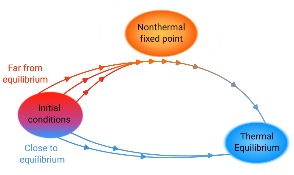
Now imagine that we have an isolated system, i.e., one that does not exchange energy with its surroundings, such as a very high-quality sealed thermos. However, instead of such a fancy thermos, the systems of interest in this case include the hottest plasmas on Earth in heavy-ion colliders, the coldest gases on Earth in an ultracold quantum gas, and the early universe. For these systems, a curious phenomenon may occur on their way to thermalisation under certain extreme conditions, which, in principle could even indefinitely delay thermal equilibrium: the approach towards a so-called nonthermal fixed point. In fact, at the Kirchhoff Institute of Physics in Heidelberg, such a nonthermal fixed point has been experimentally observed for the first time ever a few years ago using a device known as a quantum simulator.

Before understanding how this could arise, let us briefly discuss the meaning of fixed point and nonthermal in this context. Mathematically, a fixed point is a value or property that does not change under a given transformation. We can easily visualise this with the help of Fig. 2a), which shows a rotating rectangle. In this illustration, our given transformation is a rotation, and one of the edges of this rectangle is a fixed point of this transformation. No matter how we rotate, that point always remains fixed, i.e., invariant. We may also connect this to the idea of scale invariance, as seen in Fig. 2b), which is the essence of our fixed point.

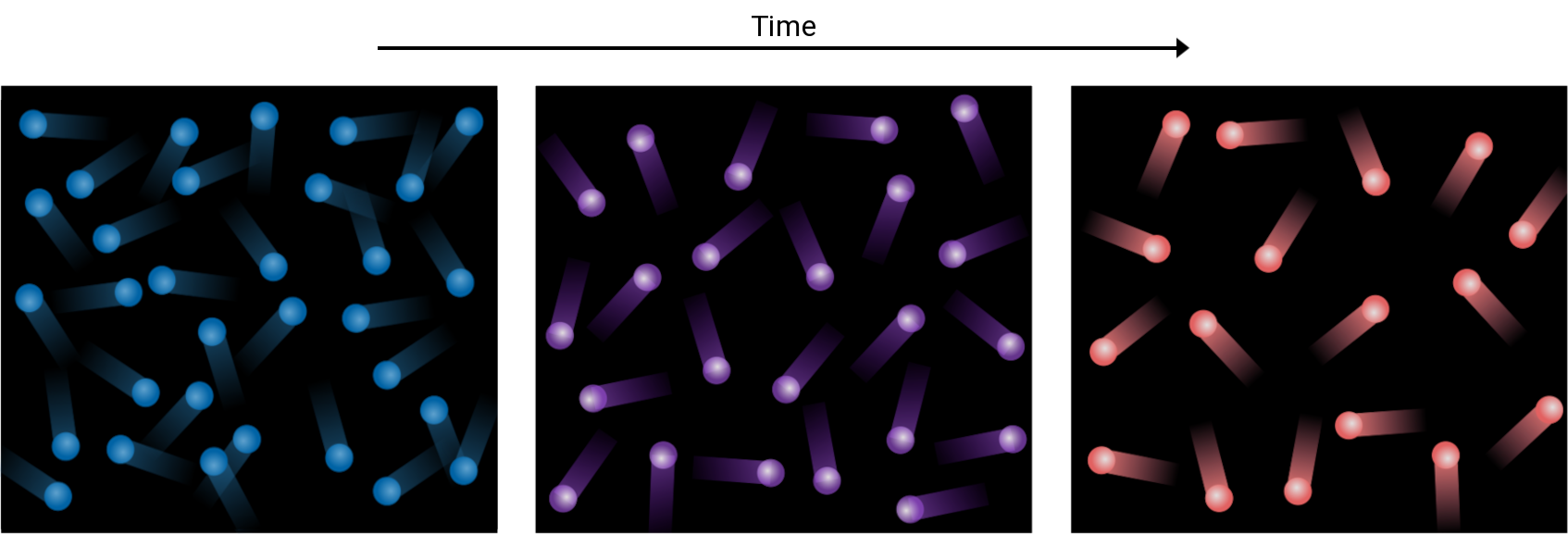
In thermal equilibrium, every process is equilibrated by its reverse process. There is no net movement of energy or particles from one place to another, and e.g., there is no group of particles that suddenly all speed up or slow down. Therefore, there is a detailed balance. Going back to our isolated system, we can, however, inject it with lots of particles and thus overoccupy it. This overoccupation is taken as the “initial condition”, namely our zero second. Such an overoccupation strongly violates the balance of equilibrium and leads to a net flux of energy and particles across different particle speeds, such that our isolated system is far from equilibrium. Yet, it turns out that after some time, this system can appear scale-invariant: we can “zoom in and out in time” and observe the same scale-invariant behaviour. Hence the notion of a fixed point, and since there is a net flux of energy and particles across different scales, which is not the case in thermal equilibrium, our system is also nonthermal.

But what kind of a physical quantity do we need to study to understand this behaviour?

For instance, we can plot a function of the total number of particles for each possible speed in our isolated system. After our initial “injection” of many particles, most particles lose speed, some others gain speed during collisions, and naturally, the shape of the plot changes with time. However, plotting multiple of these curves at different times, we see that the graphs representing the number of particles appear to “move to the left” and “shift upwards”.

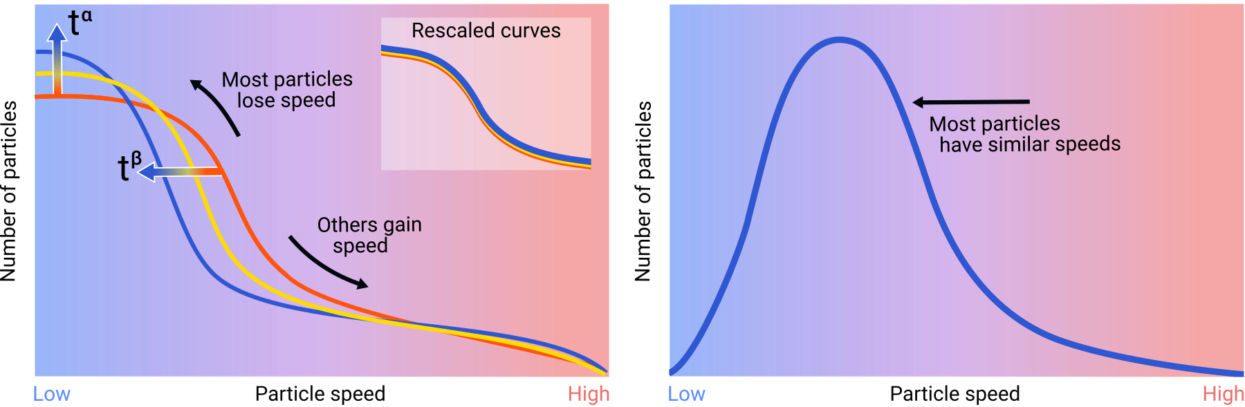
This “shifting left and upwards” such that the curves at different times all fall on top of each other is a manifestation of self-similarity, i.e., the number of particles as a function of speed shows self-similar behaviour. We can then extract the numbers, by which we shift our graphs up and left. These numbers are referred to as universal – and in fact, nonthermal fixed points are governed by laws that are universal. This means that no matter what the system consists of, we can describe it with only a small set of numbers: hot plasmas and cold gases far from equilibrium can all be described by the same laws. These universal numbers are called scaling exponents, and they are often simple numbers: for instance, $\beta= \frac 12$, and $\alpha = \frac 32$ in the plot above.

During the far-from-equilibrium universal scaling, the number of particles with low speeds increases over time: the yellow curve is higher than the orange one, and the blue curve is even higher than the yellow one. Eventually this leads to something known as a Bose-Einstein condensate, which naturally, at some point will also decay. This condensate cannot form instantaneously as particles need time to move to the lowest speeds, and similarly thermalisation cannot occur in an instant either. But what happens during this time?

Geometric Structures in an Isolated System Far From Equilibrium – Topological Defects

We have learnt that in an isolated system far from equilibrium, such as one injected with many particles, there is a subsequent universal scaling behaviour: the system is self-similar in time and space. This behaviour is “driven” by the particles losing speed and forming the condensate. However, while these slowing particles form the condensate, other structures, like topological defects, may also form in our system. The formation and dynamics of these defects represent another physical process.

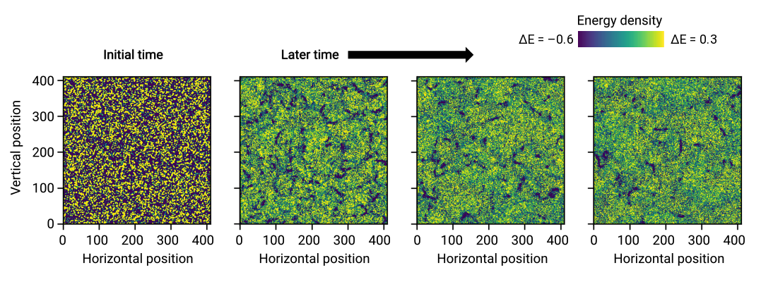
These defects are essentially disruptions in our more or less homogeneous systems, like a snag or a tear in the fabric of clothing, disrupting the pattern. For instance, they appear as distinctly low energy dips in the spatial distribution of energy density, as seen in Fig. 7. Such defects can come in different shapes and sizes, and what makes them “topological” is that they can be rigorously described in a mathematical manner using quantities from the field of topology.

Topological Defects and Nonthermal Fixed Points

One of the easiest ways to study far from equilibrium systems, nonthermal fixed points and the dynamics going on in general is by using numerical simulations. In the following, a three-dimensional lattice was used to study the behaviour of topological defects in a far from equilibrium system.

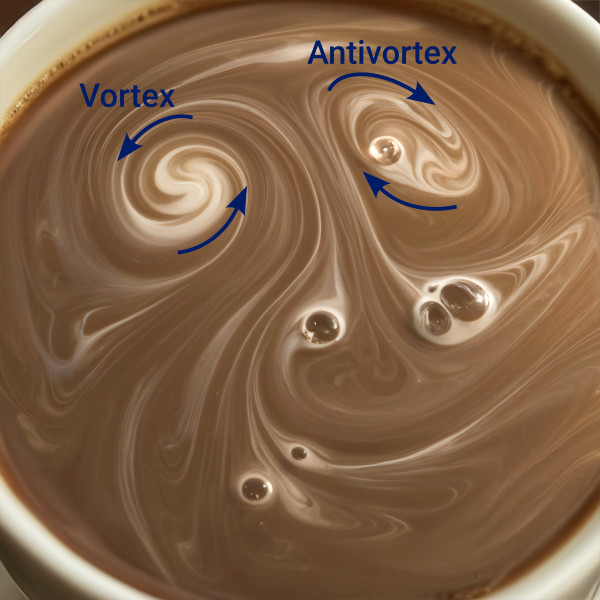
In a three-dimensional system, we can observe defects that have the structure of vortex lines or loops. A particularly suitable quantity to study them is the spatial distribution of energy density, as defects distinctly show up as “dips” there.

We know that these vortices, which circulate in a certain direction can meet antivortices, circulating in the opposite direction – and when these two meet, they mutually annihilate each other. This kind of vortex-antivortex annihilation is also known to give rise to scaling behaviour with universal scaling exponents, which has been discovered long before nonthermal fixed points. We can essentially consider these vortices as large, slow-moving “particles” for practical purposes. However, the particles that drive the scaling described in the previous section are very energetic, since we gave them a lot of energy initially by injecting many of them into the isolated system. The vortices/antivortices on the other hand are all at low energy, as we can see in the figure above. Nevertheless, there are still quite a few of them, and therefore vortices and antivortices annihilating could still display universal scaling behaviour with scaling exponents that may be different from the ¹⁄₂ and ³⁄₂ observed previously. This scaling could also coexist with the one driven by the energetic particles.

The hindrance is that the vortices are very large and slow objects. Even if we consider them to be “particles” for practical purposes, their scaling behaviour simply loses out that of the highly energetic particles, which dominate the scaling in terms of “number of particles” in Fig. 4. How can we then observe scaling due to vortices?

Fortunately, while the vortices might not show up in the total particle number function, we can still see them very clearly with our eyes. We can therefore come up with some creative “observables”, i.e., some quantities to measure or observe, to quantify this “hidden” scaling behaviour. One set of suitable observables can be borrowed from the world of topological data analysis, which is suitable for the underlying investigation because it stores a lot of information about the aforementioned defects, which are also topological.

Persistent Homology to Study Structures

Persistent homology is like a detective for exploring the patterns in data. Let us walk through a pedagogical example how this works on a two-dimensional space.

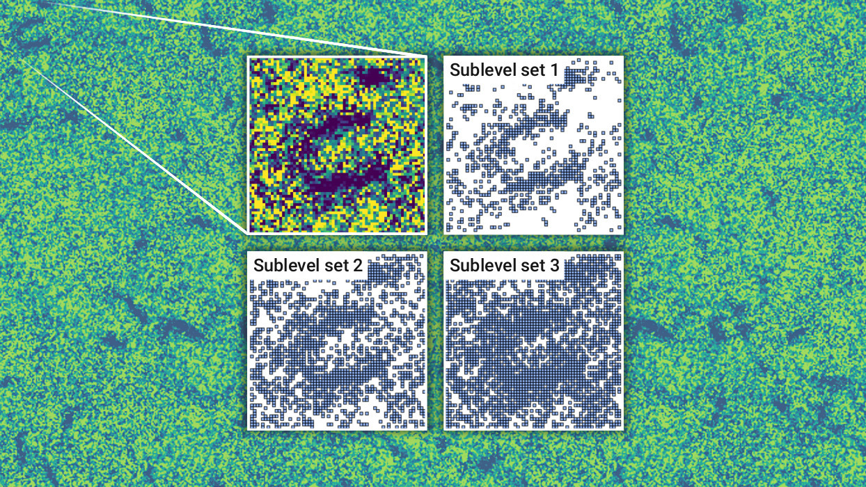
In Fig. 8 (a), energy density fluctuates from -0.6 to 0.3. Clearly, there is a horseshoe shaped vortex-line defect. Let us think of this data as a collection of tiny squares, such that these squares are arranged in layers. We examine these layers one by one through the animated figure in Fig. 8 (b): first, we fill up all the squares where the energy density is less than or equal to -0.4 in value, such that we include all the squares whose value is between -0.6 and -0.4. This corresponds to the first picture in the animation. Next, we fill up all the squares that are less than or equal to -0.35 in energy density – thus we have our second layer, and second picture in the animation. Note that this second layer includes all of the first layer, and the extra squares where energy density is between -0.4 and -0.35. In fact, these layers are called sublevel sets as can also be seen in the title image.

As we do this layering, we start to see interesting shapes emerge, such as the horseshoe. Persistent homology helps us identify these shapes by analysing how they persist across different layers. For example, if we see a blob forming in one layer and it stays there as we fill up more squares in the next layer, we can confirm it is a robust feature of the data. Therefore, persistent homology helps us see the big picture by revealing the long-lasting structures in our data. We see that the horseshoe is a robust feature of the data up to energy density 0.0.

Next, we may explore a three-dimensional grid, where each point represents the energy density at that spot. Now, this grid is like a giant Lego set, with each cube representing a particular region of space. As we sweep through different levels of energy density, some spots in the grid may become empty, creating “holes” – however, holes have a special meaning in this case: these holes are the missing pieces in our Lego structure. A Lego block, and a disconnected region made of blocks are a dimension-0 hole. If the blocks form a single hole like a tunnel passing through the grid, it is a dimension-1 hole, and a bigger hole that encloses a volume is a dimension-2 hole. These holes can be associated with so-called homology classes, hence the “homology” in persistent homology. As we move through the energy levels, holes can appear and disappear. We measure for how long they stick around, for how long they persist, by their persistence. This is akin to tracking the lifespan of different features in our grid as we change the energy density. This helps us understand the underlying patterns in energy density fluctuations, especially around areas where defects might be.

Universal Scaling of Defects and Nonthermal Fixed Points

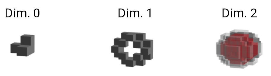
By counting these Lego blocks, we can count the total number of vortices and antivortices at any given time during the dynamics. When the topological structures are stable, they show up as Lego blocks persisting for a long enough time in our analysis. While our method cannot distinguish between vortices and antivortices, we can still count the rate of their mutual annihilation and assign a scaling exponent to it which is also universal.

It turns out, based on our persistent homology analysis, that the rate at which vortices and anti-vortices annihilate each other can be described with the universal scaling exponent $\beta_{\mathrm{top}} \sim \frac 14$ in three dimensions. This is clearly distinct from the comparable $\beta = \frac 12$ exponent that is due to the highly energetic particles losing speed and forming the condensate. Therefore, with persistent homology, we have uncovered a subdominant scaling behaviour, previously “hidden” and driven by the large and slow topological objects at low energies, while the rest of the isolated system is in a highly energetic state.

These findings not only reveal the intricate dynamics of nonthermal fixed points but also shed light on the fundamental processes governing the behaviour of isolated systems far from equilibrium. Furthermore, the results of this investigation pave the way towards understanding the richness of interactions within complex systems and highlights the importance of considering the topological contributions in understanding the universal dynamics.

Further Reading

1. Observation of universal dynamics in a spinor Bose gas far from equilibrium (M Prüfer, P Kunkel, H Strobel, S Lannig, D Linnemann, C-M Schmied, J Berges, T Gasenzer and M Oberthaler, Nature 563 (2018)).
2. Confinement in non-Abelian lattice gauge theory via persistent homology (D Spitz, J Urban, J Pawlowski, Phys. Rev. D 107 (2023)).
3. Detecting defect dynamics in relativistic field theories far from equilibrium using topological data analysis (V Noel, D Spitz, Phys. Rev. D 109 (2024)).