Mathematical Models for Climate and Weather Prediction

When planning the activities for next weekend or for your next vacation, one of the things you probably do is check the weather forecast. In doing so, you have likely noticed that most websites show you information for the next two weeks at best and that the information changes from day to day. The further out the day you are looking at, the more uncertain the prediction. At the same time, news reports talk about how the climate on Earth will change over the next decades or even centuries. If climate is more or less the average weather over a long time span, how is it possible that we can predict climate but not weather over long time spans?

Intuitively, to predict the weather tomorrow, one would rely on observations we have made in the past – for example, the weather usually only changes a bit from day to day. These common observations are also part of folklore with sayings such as “Red sky at night, shepherd’s delight. Red sky in the morning, shepherd’s warning.”

Such observations can be packaged into mathematical equations. We would call such equations a mathematical model for weather prediction. The weather forecast we see on the news is created using elaborate mathematical models for the weather systems, air pressure, temperatures and winds. These models have been developed by experts over the span of many years. They are very complicated and also very expensive to compute, requiring the use of supercomputers.

If we want to make our own versions of these predictions, we need to create a mathematical model to predict the change of temperatures in the next hours. We need to make decisions about the quantities we want to include and the details we want to consider. At first glance, it seems obvious to say that we want the most detailed and accurate forecast possible, and we should therefore include every single physical process that is known to influence the weather. However, the trade-off is that more details result in a more complex model, which is more difficult and costly to solve.

The Essence of Mathematical Modelling

More generally, mathematical modelling consists of a constant exchange between applied sciences, such as physics, biology and chemistry and mathematicians. The discovery of new natural phenomena, for example from new experimental designs, pushes mathematicians to develop new methods for abstract descriptions of the experiments. A mathematical model is a simplified representation of the real world that includes the most important but certainly not all details. You can compare it to a map of a landscape that is suitable for navigation but does not show every single tree, bench or small creek that you can find in the real world. Many of these smaller details (e.g., trees or benches) are not even of interest e.g. when we just want to find the way from A to B. Therefore, reducing complexity is not just a practical approach for making computations more efficient; in many cases, having every detail may not even be useful or desired.

Creating mathematical models relies mainly on simplifying the process that we describe and reducing it to only the most important factors.

Importantly, reducing the complexity of the real world involves expert knowledge about the process in order to determine which aspects are absolutely necessary for our understanding and which influences can be neglected. The simplifications allow us to consider a simpler representation that permits us to understand the system.

After reducing the experiment to the most important aspects and making suitable assumptions, mathematicians begin to translate those into equations.

Depending on the level of detail we decided to include, we can use different mathematical tools. An important concept for mathematical modelling is the theory of differential equations, which can for example describe how physical quantities (such as temperature and air pressure) change. We differentiate between two important types:

• Ordinary differential equations describe how a system changes in one aspect (usually time). They are suitable for describing average values (for example the average temperature). These equations are relatively easy to solve, at least on a computer, but need a lot of simplification.

• Partial differential equations can be used to describe the changes of a system in several variables and can include more different processes. They are much more complicated and the strategies to solve them, even on a computer, depend highly on the exact equation.

Using these mathematical concepts, we can come back to our weather prediction model.

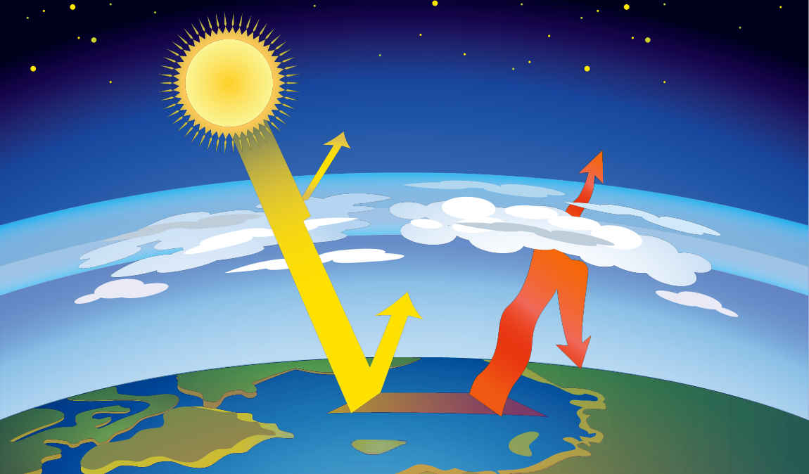
If we are only interested in the global average temperature tomorrow, we can rely on a simple model that describes the change in temperature as proportional to the difference between incoming energy (mostly solar energy from the sun) and the exiting energy. The sensitivity of the temperature to these effects can be described using a constant k. We obtain the “equation”:

Honestly, this model is of very limited use when we are trying to decide which jacket to pack for tomorrow. It does not even include the seasons, which may not have a large impact on the global average temperature but certainly change the temperature at a given location. But even though this is an oversimplified model, we could use it to approximately predict average global warming. If we allow the constant k to change, this model could even include effects like the change of the Earth’s atmosphere, which accelerate average global warming. We could use this model to predict how the global temperature increases if the Earth is 10% more efficient to retain energy, i.e. if the constant k increases by 10%. Within this simple equation, we can actually include many effects as long as we look at the average effect over the whole Earth over time. If the composition of Earth’s surface changes and reflects less heat (for example due to melting ice shields), we can decrease the amount of energy that leaves the atmosphere in the equation. Similarly, we can include average changes in the atmosphere due to climate gasses or due to more water vapor in a warmer atmosphere.

In actual practical scenarios, it would not be very ethical or useful to employ such an absurdly simple model to inform decisions about climate protection policies. It neglects effects such as that the temperatures in some regions of Earth increase much faster than in others and that good control over the average increase in the global temperature does not help if the much higher increase of temperature at the poles leads to melting of the ice caps.

If we want to include more details, we should use a more complex equation.

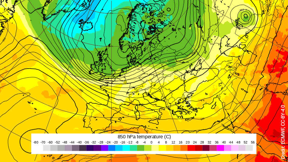
In the weather forecast on TV we have all seen how rain fronts move over continents or how the wind will move cold air from the arctic regions to Europe. If we want to understand tomorrow’s weather, we should understand how these effects move the weather fronts over the surface of the Earth. In this case, we want to understand changes in time and location. Hence, we consider a more complicated partial differential equation. This allows us to consider ocean currents and wind. Such a model would then allow us to predict the temperature at many points all over the globe.

One relatively easy partial differential equation to look at in this context is the heat equation. It describes how the heat distribution in space changes over time. The easiest effect is diffusion which describes how the heat distributes naturally until it is even in all of space. Heat naturally moves from places with higher concentration to places with lower concentration. These differences in concentration are described with the second space derivative.

For climate models, such equations could be used to study how the temperature at the Earth’s surface changes the temperature in the soil. Another important effect for climate change is the heat transfer from warmer water at the ocean surface to colder water in the depth of the oceans, which could also be described with this equation.

To obtain a more complete model, we could for example include convection, the physical process by which energy (in this context mainly heat) travels with the flow of a material but the difference in energy also induces flow in the material. In the weather context, this could model effects such as heat being transported by the gulf stream.

More Realistic Weather Models

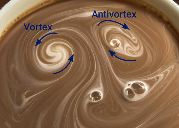
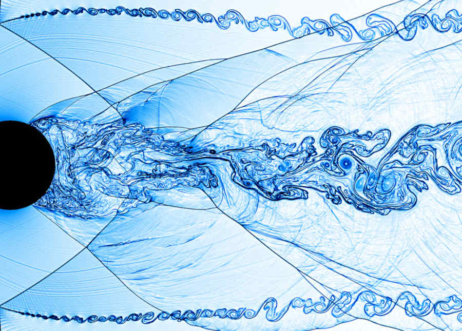
In practice, weather predictions can be made based on the Navier-Stokes equations. These equations describe how fluids (such as water or air) flow. These are an active field of study. As of today, we do not know under which conditions they have solutions if we consider such a system in three physical space dimensions (this is one of the seven Millennium problems, a list of important open problems in mathematics, https://www.claymath.org/millennium-problems/). An exact analytical theory for these equations is currently not known. This means that we cannot prove if solutions for these equations exist for infinitely long time for any reasonable initial condition, as a solution might develop very irregular behaviour after a certain time. Some results prove the existence of solutions for short time intervals. One of the most difficult aspects of the Navier-Stokes equations is turbulence, when vortices in the fluid appear on many different length scales. In mathematics, it is hard to consider all of these different scales at the same time.

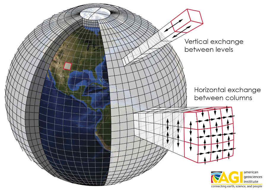
But there are algorithms for computing solutions to approximate problems by considering a discretization in time and space. Essentially, this means that we only consider the equation at fixed time points and divide up the Earth and its atmosphere into blocks. This reduces the very complex Navier-Stokes equation to a large system of equations that a computer can solve.

Connecting Models to Reality

If we consider mathematical models not just out of scientific interest but to inform real-world decisions, we need to assure that they adequately represent the real world. When creating a model, mathematicians make assumptions about the processes that we describe. A possible assumption for a weather model could be that the temperature of the Earth cannot suddenly change more than a fixed amount in one year. While it is easy to make such assumptions on paper, it is much harder to verify their correctness in the real world or to precisely measure all of the parameters influencing a model.

Remember that even the most complex mathematical model is still a simplified representation of reality. So, while it would be tempting to say that the model is objective, models are made by humans and therefore reflect the decisions of those who created them. Especially when it comes to models whose results may have real-world consequences, such as climate models, it is important to acknowledge who made the model and which aspects they deemed important. The IPCC (i.e. the Intergovernmental Panel on Climate Change) reports on the predictions of climate change do this for example by illustrating the range of possibilities in the predictions. They also include expert opinions about the reliability of the results.

Even in cases where models may encompass a range of predictions, they are indispensable and highly valuable for the applied sciences. They allow us to run digital experiments in scenarios where real-world experiments are prohibitive, be it for ethical reasons, cost or just because we cannot try out what climate change does to humanity without consequences. Modelling allows us to investigate and understand how much one influence changes a system and how uncertain we are about outcomes. If we can include possible interventions in our model, it also allows us to optimize the interventions for a certain goal, e.g. the least increase in global average temperature.

Mathematical models are an incredibly powerful tool to describe and predict real world phenomena. We just need to be aware of how a model was made and what its limitations are. What makes a good model? One that is adequate for its purpose. This purpose is very different when we compare climate to weather models. Weather prediction models are used for shorter time scales but need to provide more details. In contrast, in climate prediction we care about long time horizons but usually care less about small-scale details.

It would be very important to know if there will be a drought next summer or if we should be expecting that summers without rain are the new normal state in 50 years. But if the weather forecast for tomorrow is slightly off, and it rains when I am not expecting it, that is unfortunate but certainly not the end of the world.

Sources/further reading:

• Thompson, Erica L. & Smith, Leonard A., 2019. “Escape from model-land,” Economics Discussion Papers 2019-23, Kiel Institute for the World Economy (IfW Kiel).
• IPCC reports: https://www.ipcc.ch/report/ar6/syr/
• Millenium problems https://www.claymath.org/millennium-problems/
• Parker WS. Model Evaluation: An Adequacy-for-Purpose View. Philosophy of Science. 2020;87(3):457-477. DOI:10.1086/708691
• https://en.wikipedia.org/wiki/Weather_lore
• Schwertfeger, Benjamin. (2022). The influence of bias corrections on variability, distribution, and correlation of temperatures in comparison to observed and modeled climate data in Europe. DOI:10.13140/RG.2.2.22363.23843.