Mathematical Billiards

Do you enjoy a game of pool or billiards? I certainly do; I find it very satisfying to pocket a ball with a complicated shot following several bounces. I’m not a very skilled player, though, so I miss a lot of shots. Luckily, I can blame these failures on friction and inelasticity in the collisions, or on the unexpected interference of a different ball. You can imagine my relief when I learned of the existence of mathematical billiards!

In this post, I will describe several varieties of mathematical billiards and discuss how I use computer experiments to make progress in studying these games. The images you see partially come from Geogebra and from a piece of software I created and host on my website. More on that later; let’s dive into the first game.

Inner Billiards

Imagine you’re playing billiards, but instead of a standard rectangular table, you’re using a custom-made one with no pockets and in a shape of your choice. We can draw the shape of an elliptical billiard table for instance (see Fig. 1). This choice is just an example, however! You can use any shape at all as long as it is convex, meaning that you have a clear shot from any point on the rails to any other:

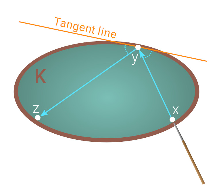
Now pick two different points at the ellipse’s boundary – let’s call them “x” and “y”. Imagine that you strike a point-like ball at x in the direction of y. It will traverse the cyan path in Fig. 1, bouncing off the wall towards a new point “z”. In an idealized, frictionless world, we can follow the path of the ball through as many bounces as we wish. The resulting sequence of chords is called a trajectory. Mathematical billiards is the study of the trajectories of balls in these idealized billiards games.

For Advanced Readers: Billiards as dynamical systems

Mathematicians like to describe “games” like this as dynamical systems. A dynamical system is a description of a “state” (in this case, a pair of points like x and y above, such that at some time the ball travels from x to y) together with a way in which that state evolves over time (in this case, the physical notion that when the ball bounces at y, it will change course and head for z).

Those familiar with the theory of dynamical systems might describe the game in the following way: billiards is a dynamical system on the space of directed chords in the body K that defines our table. The billiards map T_K is the transformation that does the operation described above: it “eats” the directed chord xy and “spits out” the chord yz, such that the chords obey the law of reflection at the point y.

Geometers who study these kinds of systems ask questions like: does K admit a periodic trajectory? That is, can one choose an x and y such that resulting trajectory retraces its steps exactly after some time?

Many mathematicians have studied this form of billiards and much is known, but there are also fundamental questions which remain open. For instance, it is not known whether all triangles admit periodic trajectories. A good reference for the topic can be found here.

Outer Billiards

Occasionally a novice billiards player like me might strike the cue ball a bit too forcefully and knock it entirely off the table. If you’ve had this experience, worry not! Mathematics is once again there for us with a game called “outer billiards.” This game no longer follows the “ordinary” rules of physical billiards (i.e. the physics of collisions on a table), but is an abstract game describing the motion of an object around a given geometric shape according to an entirely different set of mathematical rules.

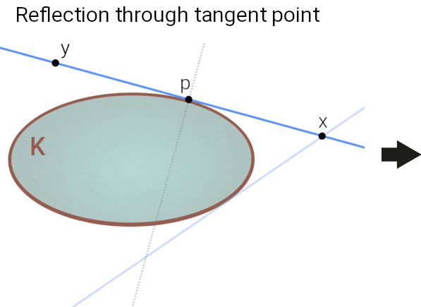
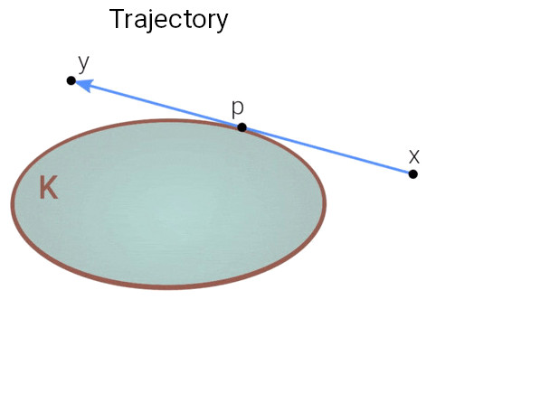
For illustration, we choose again the simple example of an ellipse. Consider a point “x” outside the ellipse and construct its two tangent lines to the ellipse’s boundary. As sketched in the animation in Fig. 3, pick one of the two tangent points (called “p” in the figure) such that the interior of the ellipse is on the left side of the blue line segment, as seen from a player located at x. Finally, reflect the player’s position x through that tangent point to obtain the new point “y”. The resulting path from x to y then corresponds to one “strike” in this modified billiard game.

Outer billiards is a new dynamical system, where a state is a point in the plane outside the table, and the evolution of the system is the map taking x to y as described above. Having arrived at y, we can repeat the same procedure again and again. The sequence of all places the “billiard ball” is going to visit in this way, when starting at x (in other words the set containing the point x, the point x is sent to, the point that point is sent to, and so on) is called the orbit of that point.

Outer billiards provide a rich field of study because there is a variety of behaviours on display. Depending on the choice of geometric shape of the body being studied, one may see very predictable behaviour, or something chaotic. The outer billiards system is very well-behaved in the case of an elliptical table: every orbit lies on an ellipse which shares its foci with the table. But tables have been demonstrated for which orbits diverge to infinity (reference).

Singularities of the Outer Billiard Map

For the rest of this post, I will predominantly be discussing cases in which the geometric shape that is being studied is a regular polygon. The attentive reader may have noticed a hole in our definition of the outer billiard map: what happens if the tangent line along which we wish to reflect x lies along a flat side of that shape? Points on one side of this line are reflected through one vertex, while points on the other side are reflected through another. There is no way to define the map for a point on the line that bridges that gap, so we will say that the map is not defined here, or that it has a “singularity at x.” When our table is an n-gon, this means we must exclude n rays (the extensions of the sides of the polygon) from the domain of the map. Apart from these singularities, however, the map is very nicely defined.

But… could it happen that a billiard ball which starts at a non-singular point eventually reaches a singular point and gets stuck? This can indeed happen. We have to call all of those starting points singular too, because we are only interested in points whose entire orbits are defined. So what does the complete singularity set look like? Here is where the computer really shines.

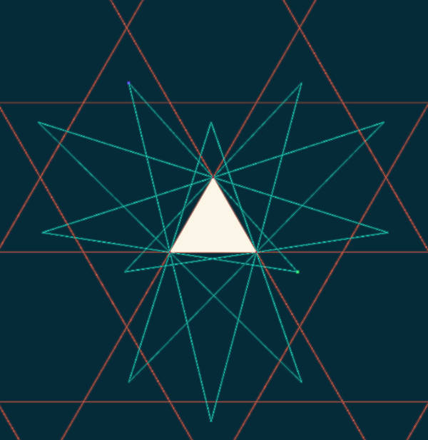
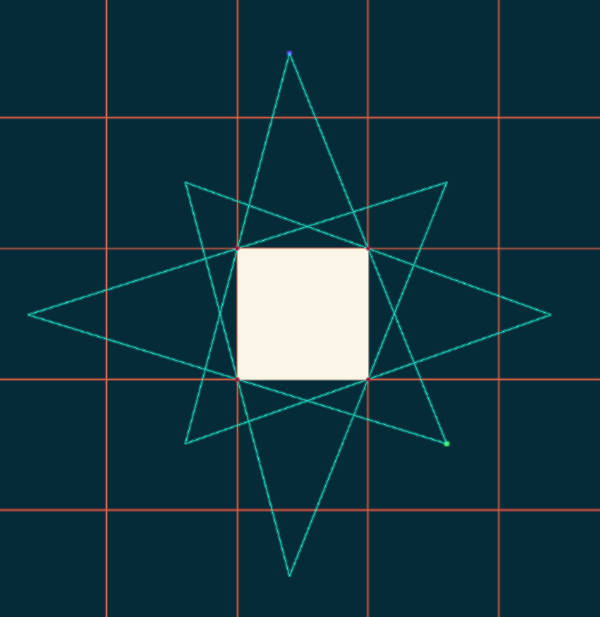
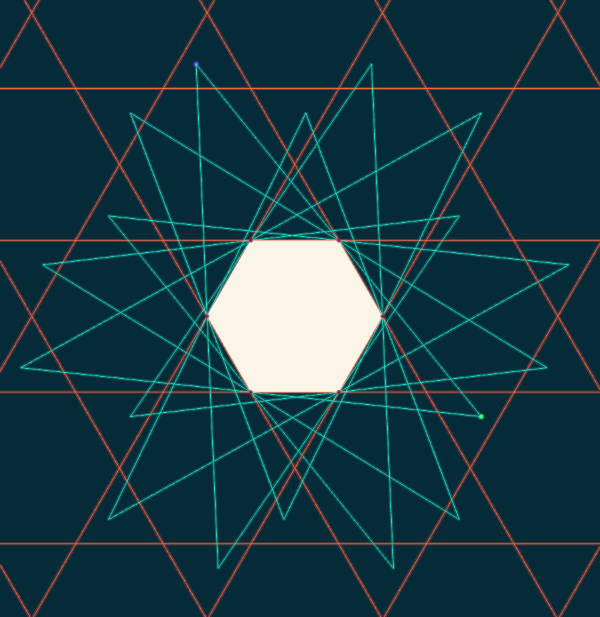
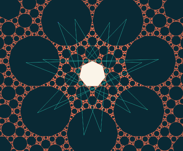
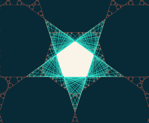
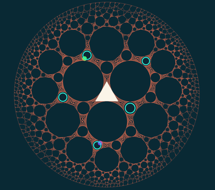
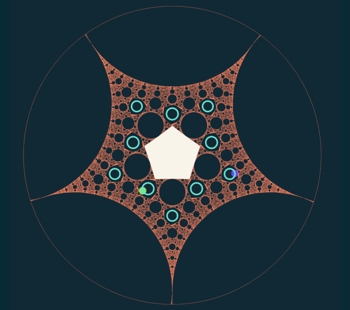
If our table shape is a regular tiling polygon (i.e., triangle, square, or hexagon), the singularity pictures are tilings of the plane (and every nonsingular point lies on a periodic orbit). But for regular polygons with other numbers of sides, the pictures we get can be much more complicated (see, e.g., Fig. 5). Some cases have been studied in detail. The pentagon has well-described fractal behaviour and non-periodic orbits, for example.

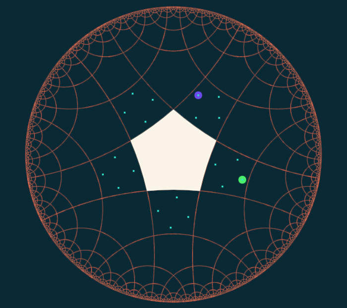
For all regular polygons, no matter how many sides they have, we can make the following observations: there are some polygon-shaped regions in the plane where there are no singularities (the dark regions in the images). If a ball starts in one of the regions, it will be sent to another and another. Sometimes, the ball may come back to the region it started in, and if that happens, then it turns out that every starting point in that region will come back to its starting point! For these reasons, we sometimes call these regions “periodic islands.” For tables of almost any shape, it is typical to observe a number of these islands together with some messier regions in between them.

For Advanced Readers: Hyperbolic Outer Billiards

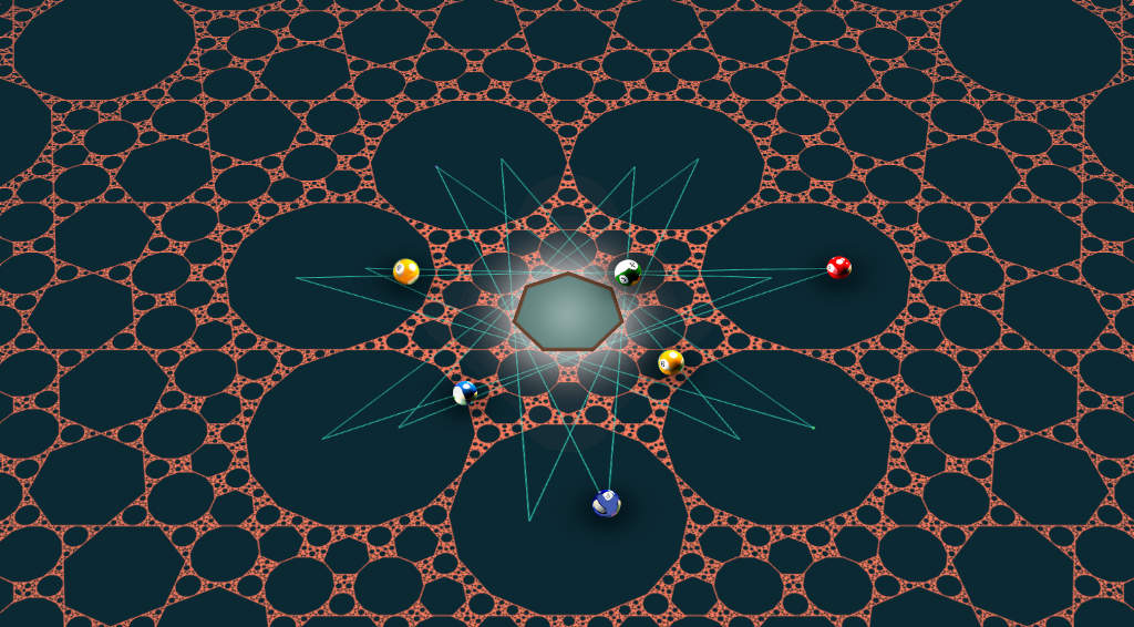
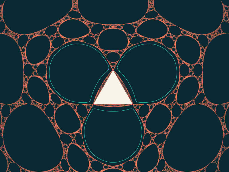
One variation of this problem I have found particularly interesting to explore is the translation into hyperbolic geometry (for a primer on this topic, see e.g. this website). A key difference for our purposes is that there is no longer a single regular n-sided polygon for each n, but an entire family of them with different side lengths. Let’s start with equilateral triangles. A typical singularity diagram appears to have circular periodic islands of various sizes, as well as smaller connected components with unknown descriptions. Perhaps these regions comprise periodic orbits? Perhaps they have some fractal structure?

But as we vary the length parameter, we might occasionally notice a striking regularity in the image. For a few very precisely chosen side lengths, the image simplifies dramatically. In fact, for any integer $k\geq 7$, we can compute a side length $\ell(k)$ with the following special property. The singularity set of a triangle with side length $\ell(k)$ looks exactly like a tiling of the plane by triangles and $k$-sided polygons, with two copies of each shape meeting at each vertex in alternating order. This result holds for all integers $n,k\geq 3$ such that $1/n+1/k < 1/2$. This tells us that in hyperbolic geometry, there is an infinite number of different regular polygonal table shapes for which all trajectories are periodic, instead of the three we know about in the Euclidean plane. For more on these tilings in general (i.e., not in the context of billiards), see Wikipedia.

I discovered this by playing with the software programme I wrote until the pattern revealed itself. Then I was able to chase down the details by hand, once I knew what to look for. To me, this is a good example of how computer experiments can lead to progress in pure mathematics.

Outer Length Billiards

Let us now return to the Euclidean plane and describe one more, slightly convoluted form of billiards. Again, consider a point x outside the table and construct its two tangent lines to it. As viewed from x, one of the lines has the table on its left. Label with p the point of tangency of that line with the table. We now construct the unique circle C which is tangent to the table at p and to the two lines, as shown:

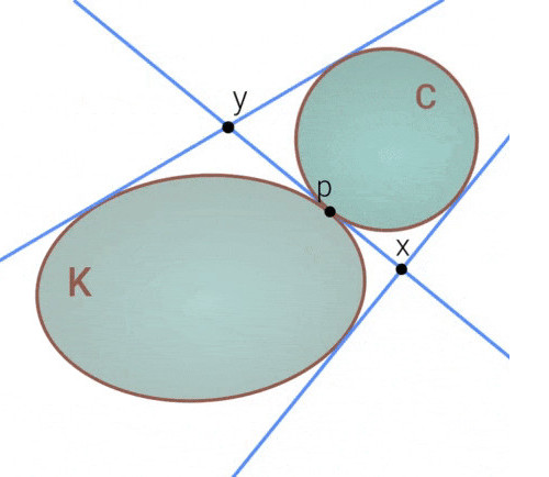
This circle actually shares three tangent lines with our table, two of which are already drawn. Construct the third to obtain the new point y, which is defined to be the intersection of the tangent line through p with the third tangent line. This game is provisionally called outer billiards with length for reasons beyond the scope of this post, and has only recently been described by Sergei Tabachnikov at Penn State and Peter Albers from STRUCTURES at Heidelberg University.

Outer length billiards is similar to outer billiards in that the map moves points along their tangent lines, but the distance travelled at each depends in a more complex way on the shape of the table. My programme attempts to draw the singularity set, defined in an analogous way as in the standard outer billiards. However, the image is more complicated. For the mathematically experienced readers, let me add that this is because the map is no longer an isometry, so the preimages of straight lines are generally no longer straight.

While every regular polygon certainly admits at least one periodic orbit in this game, little can be said with confidence at the present time about the behaviour of this system in general. However, the dynamics appear to demonstrate a fascinating combination of simplicity and complexity.

Motivation

Why do mathematicians care about problems like this? There are a few different reasons. Firstly, there is the connection to the physical world: the standard billiards models a ball bouncing in a table or a photon in a mirrored room, and outer billiards was originally conceived as a very coarse model of planetary motion. Secondly, questions of dynamics in the plane are interesting because of how much detail is hiding in a space that seems so familiar. I might say “I know Euclidean geometry like the back of my hand” but just as I might wonder to see the skin of my hand under a microscope, there is so much still to learn about the behaviour of even the simplest geometric systems. Thirdly, the experimental and theoretical tools we develop to study dynamical systems often offer returns in other areas of mathematics. The definition of a dynamical system is broad enough that many results originally formulated in the language of dynamical systems theory apply to a large and diverse collection of interesting problems.

Experiments ≠ Proofs

Lastly, I want to reflect more broadly on the various roles of computers in mathematical research. Other posts on this blog have described applications of machine learning to several scientific problems. There is also an enduring interest in computer-assisted proof methods. The 1976 proof of the Four Colour Theorem is doubtless the most famous example to date.

Because of the constraints of finite precision numerics, some mathematical results are more suited to proof by computer than others: typically, the more discrete, the better. Rigorous proofs of more continuous problems generally require (a) good bookkeeping, since each consecutive floating-point calculation magnifies numerical error, and (b) a clever way of reducing the number of required computations from infinite to finite.

Some computer-assisted proofs strike some mathematicians as unsatisfying because they show that a result is true without necessarily conveying any intuition for why. For many of us, coming to understand the why is what makes mathematics so enjoyable to study.

For the time being, my work with computers is about building intuition with no promise of rigour. When first exploring a new geometrical problem, I like to think about how to make it interactive: which parameters would I like to be able to control, which points in the figure should I be able to drag around? I try to implement the behaviour and play with the system, and get a feel for what generally happens.

Sometimes, I try to use the visualizations to look for something I expect to see, like unbounded orbits in the outer length billiards. Other times, as in the case of the hyperbolic tilings, something catches me completely by surprise. In either case, the images produced by the software are often highly suggestive of a certain behaviour, and once I have a little evidence to support a conjecture, I can turn to the chalkboard and try to work out the proof in full rigour.

Software

https://lael.dev/#/billiards