Discovering Stellar Nurseries with Machine Learning

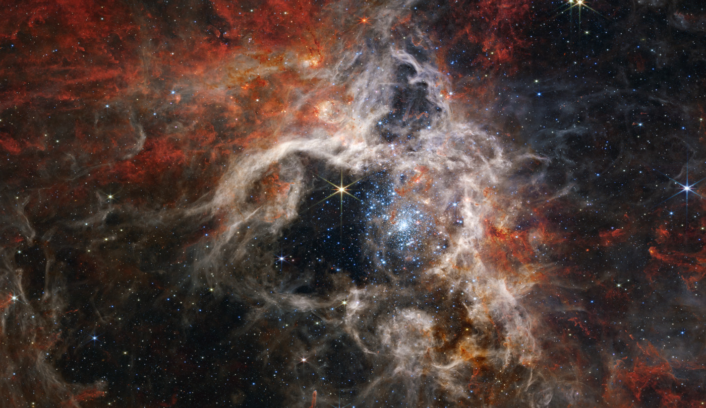
Stars are fundamental building blocks of our Universe. They bring light into the galaxies and are the very furnaces that forge most of the elements heavier than hydrogen through nuclear fusion, in particular during the late stages of their lives or, in the case of the most massive stars, their ultimate explosive demise as supernovae. Understanding the origin of stars themselves is, therefore, among the central questions of astronomical research. The star formation process consists of a complex interplay between the interstellar gas that the stars form out of and the formed stars themselves. This complexity becomes immediately evident in observations of active star-forming regions, such as the stunning banner image that shows the massive star-forming complex called the Tarantula Nebula, which was recently taken by the James Webb Space Telescope (JWST) at infrared wavelengths.

Stars are born in so-called giant molecular clouds (GMCs), aggregations of interstellar gas and dust consisting primarily of molecular and atomic hydrogen, which can reach hundreds of light years in size. A rough picture of how star formation proceeds from these enormous length scales down to those of individual stars is the following: Internal turbulence within the GMCs drives the formation of intricate substructures ranging from shock-generated sheets over filaments to cloud cores. When these substructures become dense enough, so that their internal support mechanisms (such as gas pressure, magnetic fields and small-scale turbulence) can no longer compete against their own gravity, they start to collapse, initiating the formation of entire stellar clusters – i.e. gravitationally bound systems that can contain up to thousands of stars. On the smallest (sub-lightyear) scales this collapse will eventually result in the formation of stellar embryos, protostars, which continue to accrete material from their infalling envelopes, while slowly contracting under their own gravity. This contraction is ultimately halted, when the interior of the protostar becomes dense and hot enough ($\sim 10^7~\mathrm{K}$) to ignite the nuclear fusion of hydrogen to helium, unleashing an enormous internal energy source that then stabilises the object against its own gravity – a true star is born.

As soon as the first stars have formed inside of a stellar cluster, they begin to rearrange the gas and dust of their natal cloud. In particular, massive stars greatly affect their surrounding material and can even completely destroy a molecular cloud. Aside from being powerful sources of radiation and unleashing strong stellar winds (i.e. material ejected from the stellar atmosphere), massive stars are also much shorter lived than their lower mass counterparts, such that they can turn into a supernova before their less massive siblings have even reached the conditions for hydrogen fusion. This so-called stellar feedback (i.e. radiation, stellar winds, supernova explosions) regulates the star formation process in a GMC, limiting or even cutting off the amount of mass the stellar embryos can accrete. This ultimately stops star formation altogether when the GMC is disrupted. At the same time, however, stellar feedback is also suspected to do the opposite and trigger the birth of new stellar generations by entraining material that may accumulate into new clouds, which then in turn collapse and continue the cycle.

Observing star formation is a tricky endeavour for several reasons. One of the main difficulties is the timescale of the process itself, ranging from several hundred thousand years for the most massive stars to over about 30 million years for objects such as our Sun and even up to (and above) a billion years for the lowest mass stars. This is well beyond a human lifespan (or all of human civilisation really). Consequently, all observations of star formation are only snapshots of the process, so that it is imperative to study as many still-forming stars with different masses and in varying environments as possible in order to truly piece the puzzle of star formation together. Apart from that, the actual observation of these stellar embryos is also not trivial. While the protostars themselves do emit light, primarily by radiating away the gravitational binding energy of the accreted material, they are so heavily obscured by the dust and gas of their natal cloud during the early formation stages that they are practically invisible in the optical wavelength regime and only visible in the infrared and radio (interstellar dust absorbs and scatters light much more at short than at long wavelengths). Only during the later formation stages do the stellar embyros become observable at frequencies visible to the human eye when they have already accreted and cleared out most of their surrounding material.

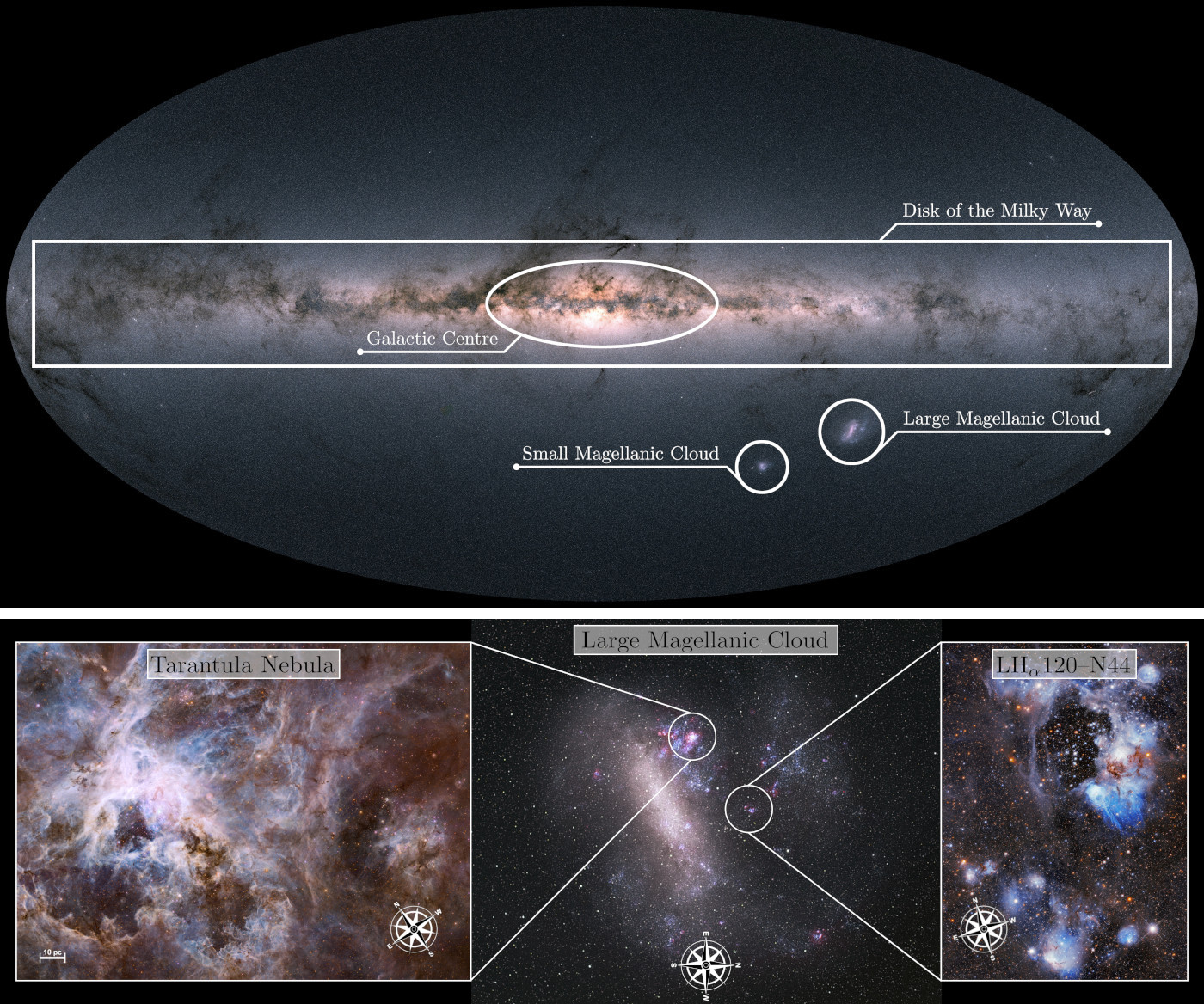
One prime location to observe star formation in action is the Large Magellanic Cloud (LMC), a companion galaxy of the Milky Way that is observable from the southern hemisphere. The LMC is characterised by an exceptional star-forming activity, hosting some of the most massive star-forming complexes in the local Universe, such as the Tarantula Nebula. Given its location below the Galactic Disk (see top panel in Fig. 1) the LMC is largely unobscured by the Milky Way’s gas and dust, unlike star-forming regions inside our galaxy, such that observations suffer much less from extinction (the attenuation of stellar light through scattering and absorption by dust and gas between the source and observer). Lastly, the LMC’s comparatively small distance of only $\sim$163,000 light years allows for observations in exquisite detail, so that modern (space) telescopes can spatially resolve even the faintest stars.

Among the main tools to study star formation (or stars in general) are photometric surveys. Photometry refers to observations where the integrated brightness of an object is measured over a limited wavelength range using filters. Although photometry certainly captures less information than a full spectrum (as spectroscopy would return), combining observations in multiple filters still allows for the characterisation of the evolutionary state of a star. One of the main workhorses for photometric observations at optical frequencies (as well as near UV and near infrared) has been (and still is) the Hubble Space Telescope (HST) because of its excellent spatial resolution and sensitivity. In recent years, several photometric surveys have been conducted with the HST that target some of the most active star forming regions in the LMC, including e.g. the Tarantula Nebula or the star forming complex LH$ _\alpha$120–N44 (see bottom left and right panels of Fig. 1 for HST images of these regions). The Hubble Tarantula Treasury Project (HTTP) and the Measuring Young Stars in Space and Time (MYSST) surveys, for instance, collected observations of more than 800,000 and 450,000 stars, respectively, in the direction of these two star-forming regions using the HST. These are, however, far from the largest photometric data sets that modern observatories are producing. For instance, the Gaia mission just recently released a photometric catalogue of more than one billion stars observed in the Milky Way.

Machine Learning Classification of Stars

Given these enormous datasets that modern observational facilities provide, there is a distinct need in astronomy for efficient algorithms to properly analyse this wealth of data. Astronomers have, therefore, increasingly turned towards applications of machine learning, which revolves around data-driven algorithms that learn from data itself to make predictions. Let us now have a look at an example application of machine learning techniques in astronomy that our team in the star formation group at the Institute for Theoretical Astrophysics in Heidelberg has worked on within STRUCTURES’ Exploratory Project (EP) A.1.

Large photometric surveys towards star-forming regions, such as the HTTP and MYSST programs, capture data of hundreds of thousands of stars. However, most of these sources do not actually belong to the targeted star-forming regions, but are instead fore- and background contaminants of the observed lines of sight. Consequently, we have to first distinguish these interlopers from the young still-forming stars that we are actually interested in. If we do not have distance measurements for the individual stars, this is, however, not an easy task and has to rely on distinguishing the evolutionary stages of the stars rather than geometric arguments. This is often the case for the LMC as distance measurements to stars in the LMC remain difficult. As the contaminants belong mostly to the greater field of either the Milky Way or the LMC itself, they are for the most part very old stars, contrary to the young sources that are actually located in a star-forming region. Unfortunately, even the distinction by evolutionary stage is not a trivial matter when relying solely on photometric observations, as there are physical effects (e.g. extinction) that can introduce ambiguity and confusion to this task.

The Support Vector Machine in a Nutshell

The Support Vector Machine (SVM) is an extension of the Support Vector Classifier (SVC), which classifies data by constructing a so-called hyperplane that best separates the classes in the training data. It does so by maximising a margin (minimum perpendicular distance from the hyperplane to the training instances) between the two classes, while allowing for a specified amount of training examples to fall on the wrong side of this margin. The left panel of Fig. 2 provides a 2D example of the SVC setup. Given a set of $N$ training instances $\mathbf{x}_i = \{x_{1,i}, \ldots, x_{M, i}\}$ of dimension $M$, each with an assigned class label $y_i \in \{-1, +1\}$, the SVC constructs a hyperplane (e.g. a line in 2D or a plane in 3D)
$$f(x) = \mathbf{x}^T \beta + \beta_0 = 0,$$

where $\beta$ and $\beta_0$ are the constants defining the plane, as the solution of the maximisation of the width of the margin $M$
$$\max_{\beta, \beta_0, \epsilon_1, \ldots, \epsilon_N} M, \,\,\,\,\,\,||\beta|| = 1,$$

subject to the constraints

$$\begin{split}
y_i \times \left(\mathbf{x}_i^T\beta + \beta_0\right) &\geq M (1 - \epsilon_i) \\
\sum_{i=1}^{N} \epsilon_i &\leq C, \,\,\,\,\epsilon_i \geq 0,
\end{split}$$

where $\epsilon_i$ indicates where a training instance $\mathbf{x}_i$ falls with respect to the margin, i.e.
$$\epsilon_i
\begin{cases}
= 0 & \small{\textsf{correct side of the margin}} \\
< 1 & \small{\textsf{wrong side of the margin (i.e. inside the grey shaded area in Fig. 2)}} \\
> 1 & \small{\textsf{wrong side of the hyperplane (i.e. wrong side of the black line in Fig. 2)}.} \\
\end{cases}
$$

Here $C$, bounding $\sum_i\epsilon_i$, denotes the budget for allowed margin violations. Once the solution hyperplane to this optimisation problem is found, the SVC is given by
$$G(\mathbf{x}_*) = \mathrm{sgn}\left(\mathbf{x}_*^T \beta + \beta_0\right),$$

where $\mathrm{sgn}$ denotes the sign function.

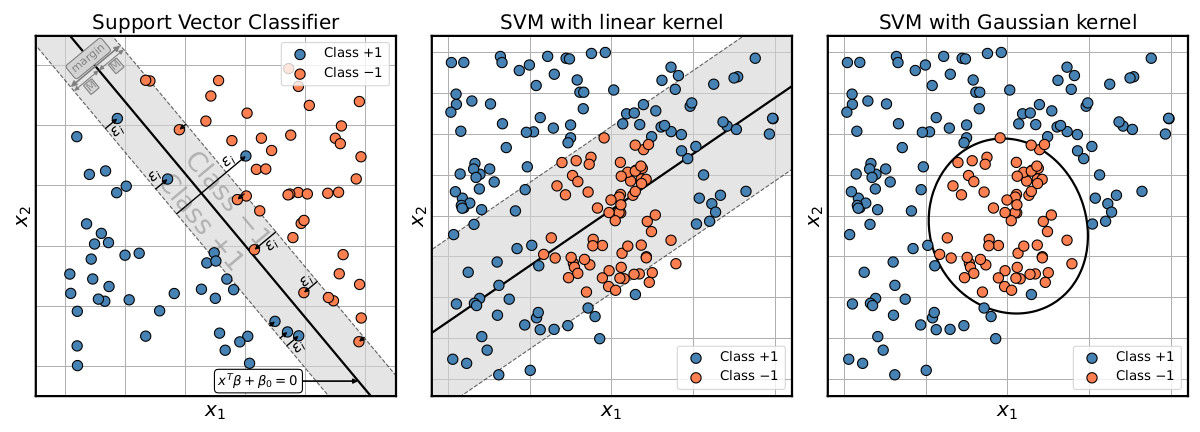
The SVC works well for classification problems where the class divide is reasonably approximated by a linear boundary (left panel in Fig. 2). For more complex, non-linear class boundaries, the SVC quickly falls short (centre panel in Fig. 2).

This issue can be mitigated by embedding the classification problem in a higher dimensional space, where the classes are again separable by a linear boundary (translating to a non-linear decision boundary in the original space). This is the basic idea of the SVM. Here the SVM approach makes use of the fact that the SVC optimisation problem can be expressed in terms of inner products (making use of so-called Lagrangian duality, such that e.g. the solution function can be expressed as
$$f(\mathbf{x}) = \beta_0 + \sum_{i=1}^{N}\alpha_i y_i \left<\mathbf{x}, \mathbf{x}_i \right>,$$

where $\alpha_i$ is only non-zero for training instances that either lie directly on the margin or violate it (the so-called support vectors). The SVM uses this property to perform the transformation to a higher dimensional space only implicitly by means of the kernel trick, substituting the inner product by a kernel function $K(\mathbf{x}, \mathbf{x}_i)$. This is not only computationally efficient, but also allows transformations to infinite dimensional spaces when employing for instance a Gaussian kernel. With this approach the SVM (with the right kernel) can tackle even complex non-linear problems, where the basic SVC fails (see right panel in Fig. 2).

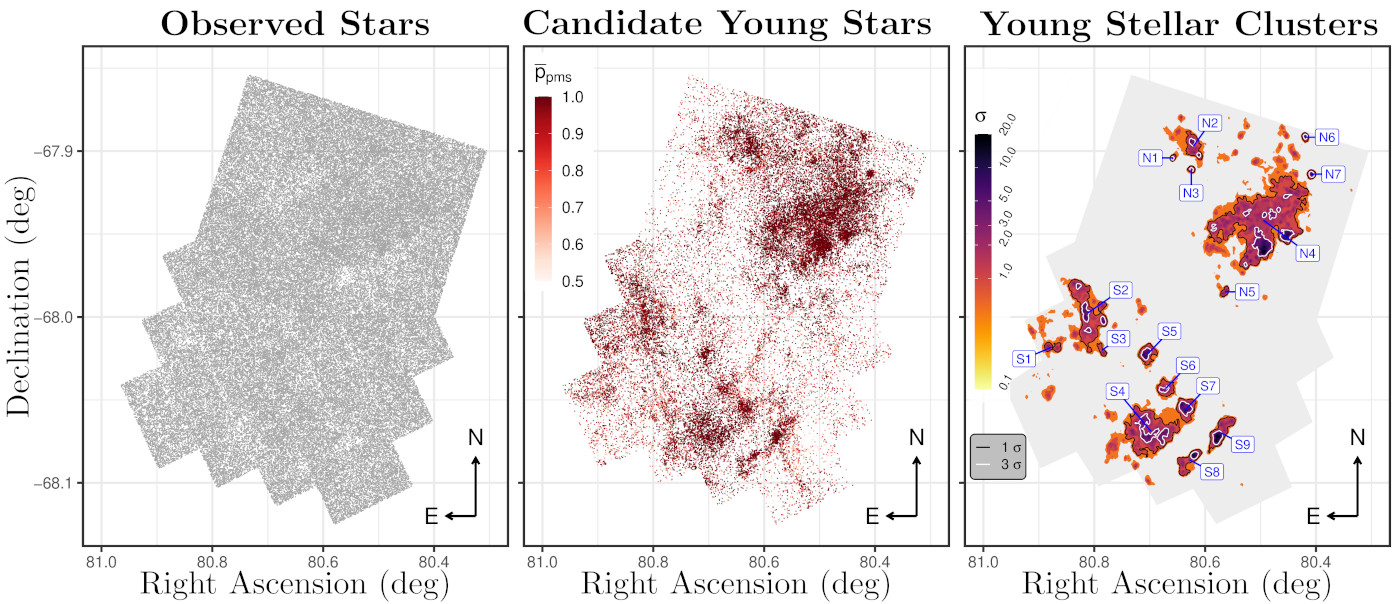
To tackle this task for the observational data of the HTTP and MYSST surveys, we can formulate it as a two-class classification problem, distinguishing only between young, still-forming stars and “old stars”, where the latter label includes all evolutionary stages after the onset of central hydrogen burning. Using methods from e.g. classical machine learning (i.e. not involving neural networks), one can then perform the distinction between these two classes. Our work, for example, employed a combination of a support vector machine (see the SVM in a nutshell box for a quick summary) and a Random Forest. The following shall outline the application of this approach to the MYSST data of LH$_\alpha$120–N44 (see the left panel of Fig. 3 to get an idea of the volume of the data that needs to be disentangled here).

Both the SVM and the Random Forest are methods that fall under the supervised learning category of machine learning models. This means that these algorithms require a labelled training data set, which links the observables (e.g. the measured photometric brightness) to the target parameters (e.g. class label), in order to learn how to perform the specified classification task. In our approach this training dataset is created by selecting a subset of the photometric catalogue of the MYSST survey (consisting of 17,000 sources) that corresponds to a single star-forming cluster (and its vicinity), where it is easier to manually assign the class labels. On this labelled set of examples, the chosen models are then trained to distinguish the old from the young stars and rigorously tested, before they are unleashed onto the entire 450,000 sources of the complete MYSST catalogue.

The centre panel of Fig. 3 shows the fruit of this labour, revealing the young “needles in the haystack” of the MYSST data and the rich clustering structure of these still-forming stars, most of which reside alongside the edges of N44’s characteristic super bubble (a structure formed by the stellar feedback of the massive stars inside the bubble, see bottom right panel of Fig. 1). In total our analysis identifies $\sim$26,700 candidate young stars in this star-forming complex. Making use of a nearest-neighbour-density based clustering approach, the structure of star formation in N44 can then be further quantified, finding 16 prospective candidates for star-forming clusters. With this data our team within STRUCTURES is now moving on to characterising the identified young stellar candidates (i.e. determining their ages and masses) with the goal of drawing a comprehensive picture of the star formation history of N44 and gaining new insights into the interplay between stellar feedback and the process of star formation.

References