Visualizing Topology and Geometry with a Connection to Physics

This post was originally published by the Heidelberg Experimental Geometry Lab (HEGL, see the HEGL Blog) and is featured as a guest article with kind permission by the authors.

Topology and geometry are important concepts in mathematics and physics. Especially in theories like general relativity, they have a direct impact, as the spacetime description of a system is already quite geometrical.
To highlight the difference between the two concepts, let’s look at a simple two-dimensional disc first. An interactive visualization of it can be found here, including several operations you can perform. For example, you can push and stretch the centre of the sphere up and down, or bend and twist the disc around.

These operations can be performed in a smooth and continuous way; we would say that the geometry of the object is changed, but not its topology. This can be seen by trying to contract the disc continuously to a point. It always works for the disc, no matter if the disc was deformed or not.
If we punch a hole in the middle of the disc instead, we have performed a non-continuous operation. This turns the disc into a CD-shape, known as an annulus (see Fig. 1b).

We can perform the same twists and deformations again, but if we try to retract the annulus to a point, a small circle will always be left over. This circle cannot be retracted to a point in a continuous manner, which shows that, topologically, the disc and the annulus are different.

The lesson is that expanding, stretching, twisting, i.e., continuous deformations, do not change the topology of a space, but cutting or punching a hole into it do. In that manner, the topology of an object represents more the underlying structure of a space (which in two dimensions can be reduced to the question of how many holes exist) or in other words, a more global perspective of an object.

Geometry, on the other hand, is a more subtle description of how much a space twists and curves. It gives a local perspective on properties like distance measurements and curvature.

Short digression: Metrics in Riemannian Geometry

An important tool in geometry is a (Riemannian) metric [1]. A metric is, in simple words, a ruler, i.e., it allows us to measure distances between points and angles at a given point. For example, on a flat sheet of paper, the distance of points can be measured by looking at the difference of the $x$ and $y$ coordinate. In general, this information can be nicely packaged into a metric, which is usually written as

$$ds^2 = dx^2 + dy^2,$$

where “$\text{d}x$” and “$\text{d}y$” represent infinitesimal changes in the respective coordinate direction and “$\text{d}s$” stands for an infinitesimal change in the total length.

More generally, given some local coordinates $(x,y)$ on a small patch of our space, a metric takes the form

$$\text{d}s^2=f(x,y)\,\text{d}x^2 + g(x,y)\,\text{d}x\text{d}y + h(x,y)\,\text{d}y^2,$$

where the functions $f$, $g$, and $h$ encode information about how curved the space is.

Using this description, let’s now look at a physical example that showcases geometry and topology: a wormhole. There are different examples of wormholes; here we have chosen the so-called Ellis wormhole, named after Homer G. Ellis, which was also independently described by Kirill A. Bronnikov at the same time [2]. The spacetime can be described by the following metric:

$$\text{d} s^2 = -\text{d} t^2 + \text{d} \rho^2 + (\rho^2 + a^2)\, \text{d} \Omega^2,$$

with the parameter $a$ describing the width of the central hole, $t$ representing time, $\rho$ a coordinate, and $\text{d} \Omega$ the angular part of the volume element, which can be expressed with two further coordinates $\theta$, $\phi$ as $ \text{d} \Omega^2 = \text{d} \theta^2 + (\sin(\theta))^2\text{d} \phi^2.$

As a solution to the equations of general relativity, this represents a four-dimensional space. To find a way of displaying this as a two-dimensional object in a three-dimensional surrounding space, we need to fix two coordinates: we take the equatorial cross-section, which is given by $t=0$, $\theta=\frac{\pi}{2}$. The metric then reduces to

$$ \text{d} s^2 = \text{d}\rho^2 + (\rho^2 + a^2)\, \text{d} \phi^2, $$

where the coordinate $\phi$ describes the position on a horizontal circle cross-section, and $\rho$ is the distance from the central circle of the throat. To find a parametric description from this, a bit more work has to be invested. First, we change the coordinates slightly, then we compare them to a known coordinate description. Change to $r^2 = \rho^2 + a^2$, which gives

$$ \text{d} s^2 = \frac{\text{d} r^2}{f(r)} + r^2 \text{d} \phi^2, $$

with $f(r) = 1 - \frac{a^2}{r^2}$.

Cylindrical coordinates $(r,\phi,z)$ should be suited for this problem from a symmetry perspective. The standard metric (ruler) of the three-dimensional flat space is given in cylindrical coordinates by

$$ \text{d} s_\text{cyl.}^2 = \text{d} z^2 + \text{d} r^2 + r^2 \text{d} \phi^2. $$

Now viewing the coordinate $z$ as dependent on $r$, i.e., $z=z(r)$, we can write this as

$$ \text{d} s_\text{cyl.}^2 = (1+z’(r))\,\text{d} r^2 + r^2 \text{d} \phi^2. $$

By simple comparison, we derive the following differential equation

$$ 1 + z’(r) = \frac{1}{f(r)} = \frac{r^2}{r^2 - a^2}, $$

which can be solved by direct integration. The result is

$$ z(r) = a \cdot \cosh\left(\frac{r}{a}\right) . $$

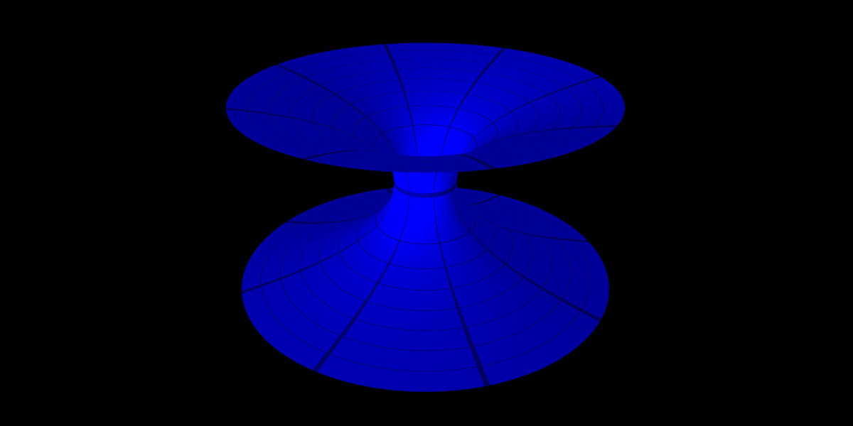
This can then be visualized, which can be found here.

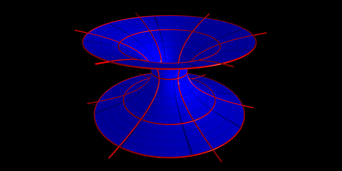
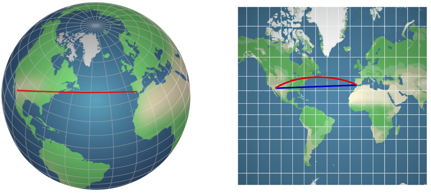
The view on the blue wormhole is a view from outside the spacetime, i.e., an observer in that spacetime would see it very differently. Grid lines on the object show how deformed it is. The parameter $a$ of the wormhole can be changed in the interactive visualization. Knowing the metric of this space, it is also possible to calculate so-called geodesics, which are the shortest paths connecting two points. This can be seen as a generalization of straight lines in flat space. A lot can be learnt from examining the geodesics of a given space. Some simple geodesics of the wormhole can be displayed in the visualization (red lines in Fig.3), but more elaborate solutions do exist [2].

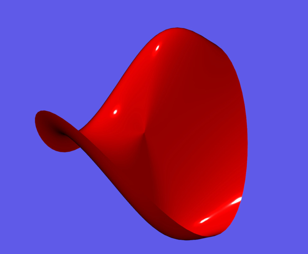
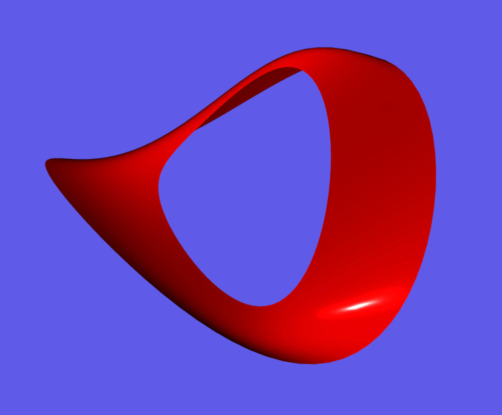
Wormholes represent substantial changes to a spacetime (topological changes), which can be seen when the wormhole connects two parts of a spacetime that would have previously been disconnected. The following is a 3D print produced at HEGL, which shows just such a scenario (you can read more about such things in [3]):

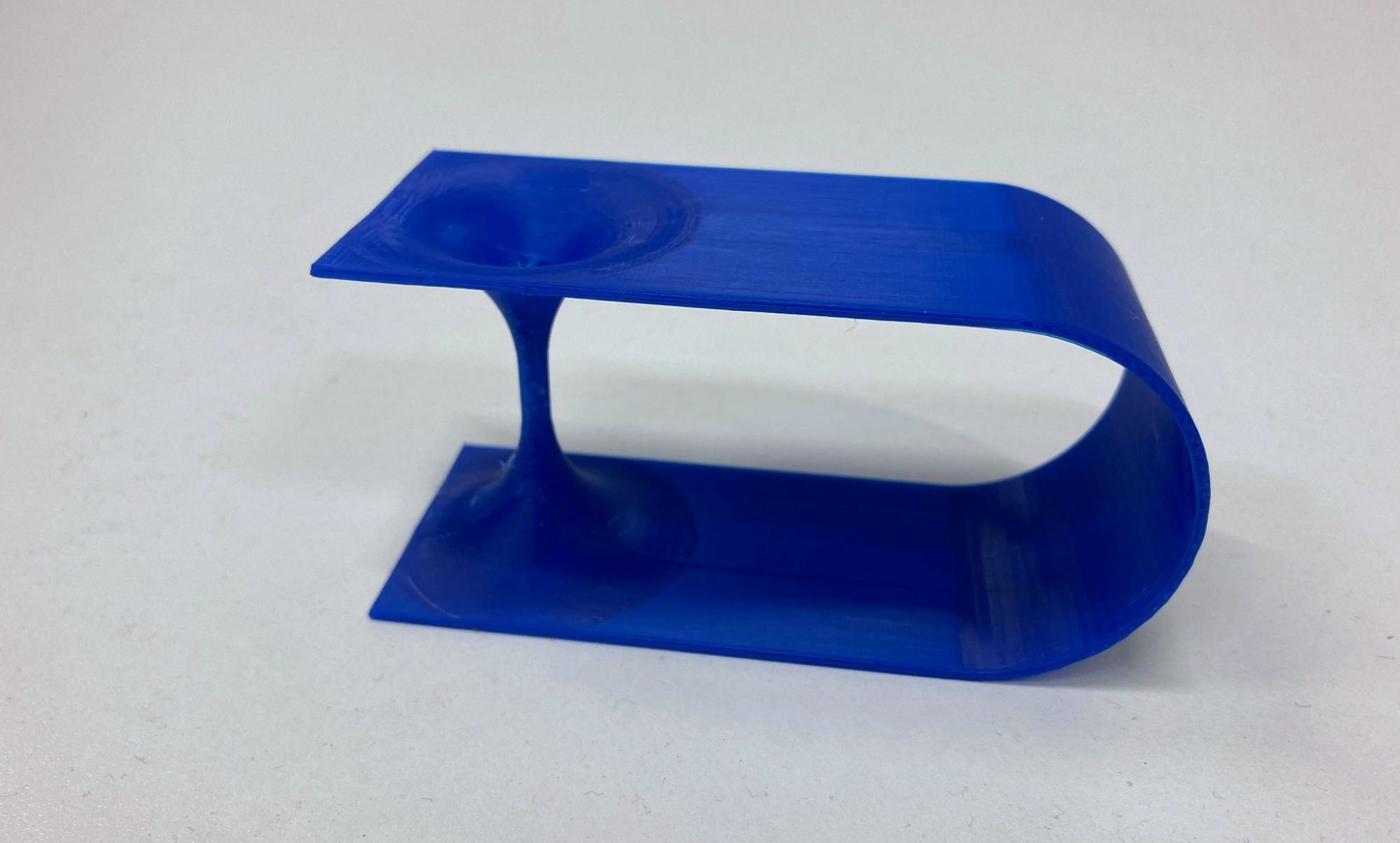
Imagine a person on the top, close to the wormhole. Going to the bottom part of the object would usually only be possible the long way around, via the right part of the bridge. But now that the wormhole is in there, a shorter path exists.

Have fun playing around with the visualizations, or drop by the HEGL lab if you want to see the 3D print. If you want to know more about how a wormhole looks like to an observer living inside the spacetime, check out [4].

About Heidelberg's Experimental Geometry Lab (HEGL)

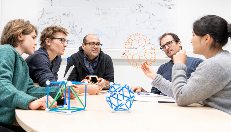
The Heidelberg Experimental Geometry Lab (HEGL) is a dynamic and vibrant community that brings together researchers at all levels to learn and exchange on topics such as mathematics research, experimental mathematics, math visualization, and applications of geometry to other fields like machine learning. HEGL is an inclusive and inviting space for all to learn and have fun.

References:

1. Wikipedia: Riemannian metric
2. Wikipedia: Ellis Wormhole
3. Wikipedia: Einstein-Rosen bridges
4. arXiv: Visualizing Interstellar’s Wormhole