Science CSI

Deduction and Inference

In science, truth can take two forms. First, there is mathematical truth, where statements are deemed true if they’re derived in a logically consistent way from fundamental axioms – and if these axioms are free of contradiction. Second, things can be true empirically, meaning that they are consistent with an experiment and that the experiment is reproducible. The process of deriving statements from axioms is referred to as deduction, and making statements about physical laws based on experimental data is called inference. Sometimes, I like to think of the scientific process of inference and deduction as if a detective visits a crime scene: There are different hypotheses at work, which need to be logically consistent, and they can be tested against the traces found at the crime scene, sorting out the empirically inconsistent ones. The famous detective Sherlock Holmes really does both: He formulates hypotheses about the crime using deduction, and isolates likely conclusions from observations by inference, despite the fact that his author Arthur Conan Doyle calls the entire process deduction.

Evidences and Hypotheses

Of course, nature is not perfect as all observations come with some intrinsic amount of uncertainty: Observations are not perfect, circumstances are out of the control of an experimenter, and signatures could have been generated by chance unrelated to the physical process under investigation. To stay in the picture of a crime scene analysed by Sherlock Holmes, there is never a smoking gun signature from which one infers one hypothesis with absolute certainty. And this, ultimately, is the reason why the empirical branch of the scientific process is necessarily statistical.

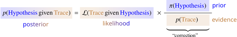
Ideally, one would like to be able to quantify the probability of a hypothesis based on the observed data (“trace”), which we can denote as $p({\color{blue}\mathrm{Hypothesis}} \, \mathrm{given} \, {\color{brown}\mathrm{Trace}})$. This measure, which takes the examination of data into account, is called the posterior probability, as opposed to the prior probability $\pi({\color{blue}\mathrm{Hypothesis}})$, which represents our initial knowledge or expectations and thus already exists even before the crime scene was scrutinised. If one reaches a very high degree of posterior probability for a certain hypothesis, its truth is established “beyond a reasonable doubt”.

Here, criminology and science differ a lot! If a detective fails to provide enough evidence to single out a certain hypothesis, one needs to fall back on the null-hypothesis: All citizens are by default innocent, and their involvement in a crime needs to be proven at low levels of uncertainty. This is a relic of ancient Roman law: in dubio pro reo, in doubt in favour of the accused, is not a statement of clemency from the side of the authorities, but an expression of the failure of the criminal investigator to amass enough evidence and of the falling back onto the null-hypothesis.

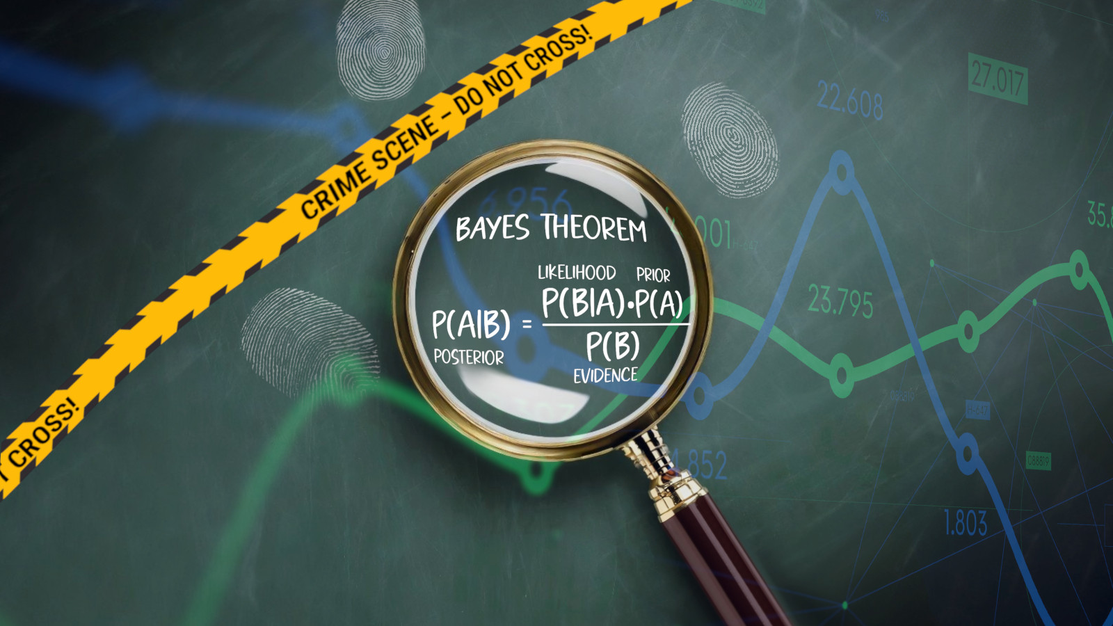
In science, all theories are innocent in the sense that they’re not contenders for a physical explanation, with the exception of a few lucky ones that are competing for being a proper fundamental law of nature. But in both cases one cannot access the posterior probability directly. This is because we do not measure probabilities. Theoretical calculations, on the other hand, may tell us how likely it is to observe this particular data given a certain hypothesis, a quantity we denote by $\mathcal{L}(\mathrm{\color{brown}Trace} \, \mathrm{given} \, \mathrm{\color{blue}Hypothesis})$. This is where Bayes’ theorem comes into play.

Scientific reasoning with Bayes’ theorem

Bayes’ theorem makes a statement about the posterior probability on the basis of the likelihood, informing us about the probabilities of possible hypotheses taking the observations into account:

At the heart, Bayes’ theorem is a statement about conditional probabilities: When the random variable (e.g. the uncertain data) is interchanged with the condition in transitioning from the likelihood to the posterior, one needs to apply a correction involving the prior distribution and the Bayesian evidence. Clearly, this correction factor is not equal to one, so it matters for computing the posterior. In general the probability of a hypothesis given the trace is not the same as the likelihood of the trace given the hypothesis.

To illustrate this point clearly, one can easily imagine that only around a billionth (≃ 10^-9) of all catholics are popes, but 100% of the popes are catholic!

For Advanced Readers: The Mathematics of Bayes' Theorem

In mathematical terms, one could argue by looking at the joint probability that the trace and the hypothesis (either innocent or guilty) appear at the same time. This could either be reached by selecting the trace first at probability $p(\mathrm{\color{brown}Trace})$, followed by picking the hypothesis at conditional probability $p(\mathrm{\color{blue}Hypothesis} \, \mathrm{given} \, \mathrm{\color{brown}Trace})$ – or, equivalently, the other way around:

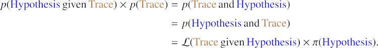
Now divide both sides by $ p (\mathrm{\color{brown}Trace}) $ to get Bayes Theorem.

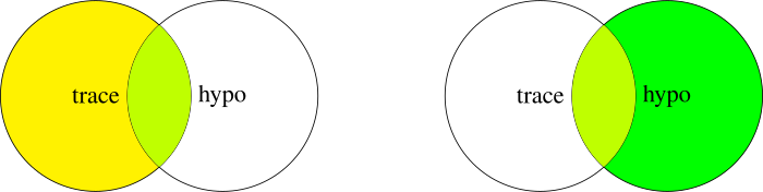
Personally, I think that this two-step selection process with associated probabilities explains Bayes’ law very well, but for clarity we can show this with Venn-diagrams acting on sets, too. Here, the conditional probabilities $p(\mathrm{\color{blue}Hypothesis} \, \mathrm{given} \,\mathrm{\color{brown}Trace})$ and $\mathcal{L}(\mathrm{\color{brown}Trace} \, \mathrm{given} \, \mathrm{\color{blue}Hypothesis})$ are clearly not identical because they operate on different pre-selections (the yellow set corresponding to $p(\mathrm{\color{brown}Trace})$ and green set representing $\pi(\mathrm{\color{blue}Hypothesis})$, respectively), even though combined with those pre-selections (and only then!), they lead to identical results (the lime-coloured intersection, corresponding to $p(\mathrm{\color{brown}Trace},\mathrm{\color{blue}Hypothesis})$):

Turning again to criminology, one can apply these concepts in an argument following this outline: imagine a criminal trial where a forensic expert analyzes a piece of evidence, let’s say a rare type of fabric fiber found at the crime scene. The expert testifies that this fabric fiber matches the one found in the suspect’s possession. The prosecution argues that this highly specific match strongly suggests the suspect’s guilt.

In this scenario, the prosecutor is emphasizing $p(\mathrm{\color{brown}trace} \, \mathrm{given} \, \mathrm{\color{blue}guilty})$, the probability of observing the fiber match given the suspect is guilty. Let’s say this match has a high likelihood. However, to truly assess the significance of this evidence, we must consider also $\pi (\mathrm{\color{blue}guilty})$, the prior probability of the subject being guilty. Let’s assume that, based on general crime statistics and other evidence, the prior probability of guilt is relatively low. In that case, even strong evidence may not be enough to establish guilt beyond a reasonable doubt.

In fact, in would be a procedural misconduct in a court to ignore Bayes’ theorem and to assume that a small likelihood $\mathcal{L}(\mathrm{\color{brown}trace} \, \mathrm{given} \, \mathrm{\color{blue}innocent})$ implied a small probability $p(\mathrm{\color{blue}innocent} \, \mathrm{given} \, \mathrm{\color{brown}trace})$, and to perfidiously continue that the probability $p(\mathrm{\color{blue}guilty} \, \mathrm{given} \, \mathrm{\color{brown}trace})$ would then be high! (Well, actually, the last statement is mathematically correct, but uses the wrong previous argument that ignores Bayes’ theorem.)

Bayes’ prior

All argumentation using Bayes’ theorem hinges on the knowledge of the likelihoods $\mathcal{L}$ and the prior probability $\pi$. The likelihoods result from the knowledge of the CSI-team (or the scientists) as they need to be able to quantify the probability at which a trace (or a data point) is generated, in both cases of an innocent and a guilty person. The prior $\pi$ is a more complicated issue: Ideally, the trace is only one puzzle piece and the prior can be set to the posterior probability incorporating the knowledge gained from all other traces, except the puzzle piece we are currently considering. If that’s not the case, there are fantastic arguments for choosing fair priors, i.e. priors that do not bias the subsequent inference steps in an unjustified way: Already Laplace formulated this as the “principle of insufficient reason”: One has to consider all hypotheses as equally possible in the absence of evidence to the contrary. Laplace’s argument was put on solid foundations by the statistician Jaynes, who quantified the amount of randomness of random processes with entropy measures, and constructed entropy-maximising prior distributions: In the simplest case the entropy-maximising prior is the uniform prior, and personally I find it striking that Laplace felt a result that was formally established only about two hundred years later.

Summary

Scientific and criminological reasoning uses Bayes’ theorem for making an assessment about the probability of a hypothesis given observed data. Bayes’ theorem is a statement about conditional probabilities and combines the prior probability of a hypothesis with the likelihoods that the data occures under the assumption of a certain hypothesis. Inclusion of the prior and normalisation by the evidence is essential, otherwise the posterior probability is misestimated.