A Bayesian Language for Modeling and Simulation

This is the first part of a series of blog posts on the topics of Bayesian models and statistical inference with neural networks. The series is a simplified summary of a scientific overview article, and intended to provide a glimpse into some of our recent conceptual and methodological work on bridging the gap between “classical” statistics and artificial intelligence (AI) research.

With the surge of probabilistic modeling, more and more branches of science subscribe to the use of Bayesian models. However, the term Bayesian model is highly overloaded and used to describe a wide range of entities with potentially very different properties and requirements. Moreover, modern Bayesian models are more than just the colloquial likelihood and a prior – rather, they resemble complex simulation programs coupled with black-box approximators, interacting with various data structures and context variables. Accordingly, two notationally similar Bayesian models may have totally different structural properties and utilities. Without clearly communicating the latter, a discussion about the relative merits of Bayesian models only contributes to the conceptual entropy in quantitative research.

In addition to sustaining a multiplicity of meanings, different Bayesian models exhibit different strengths and weaknesses, so evaluating these holistically can be quite a challenging endeavor for practitioners.
Thus, let us take a shot at the two fundamental questions alluded to above:

1. What is a Bayesian model?
2. What makes a good Bayesian model?

Providing satisfying answers to these two questions is no easy task and our answers should be treated more like conceptual blueprints than ultimate solutions. In this post, we will take a partial look at the first question concerning the identity of Bayesian models. At a high level, the basic building blocks of Bayesian model classes are probability distributions (P), approximation algorithms (A), and observed data (D). These components can be combined in various ways, leading to Bayesian model classes with different properties and utilities. In this first post, we discuss the nature of P models, as they represent an indispensable component for all model classes.

P Models

Let $y$ represent all observable quantities (i.e., data, observations, or measurements) and $\theta$ represent all unobservable quantities (i.e., parameters, latent states, or system variables) in a modeling context. P models are defined through a joint probability distribution $p(y, \theta)$ over all quantities of interest. In Bayesian analysis, we assume that everything is subject to randomness, so we embrace uncertainty by associating each quantity with a probability distribution. Using the chain rule of probability, the joint distribution factorizes into a likelihood $p(y \, | \, \theta )$ and a prior $p(\theta)$

$$ p(y, \theta) = p(y \, | \, \theta ) \; p(\theta). \label{eq:joint_fact} $$

In Bayesian analysis, the likelihood encodes our assumptions about the statistical behavior of a phenomenon and the prior incorporates prior information about the parameters. This conceptually simple factorization serves as the basis for all further Bayesian model classes (e.g., PD or PAD), which we will discuss in the next post.

Not all P models are created equal, but most are built to mimic a real-world process or a system whose behavior we can observe or measure. Thus, a P model defines a probabilistic recipe for creating synthetic data, but does not include actual “real” data (yet). In other words, P models represent simulation programs constrained by prior knowledge about the simulation parameters $\theta$. One example for such models are climate change simulations, which aim to elucidate what-if scenarios (e.g., business-as-usual vs.~behavioral and industrial change). Another example are the epidemiological models used to inform government policies during the first weeks of the Covid-19 pandemic, when little actual numbers existed.

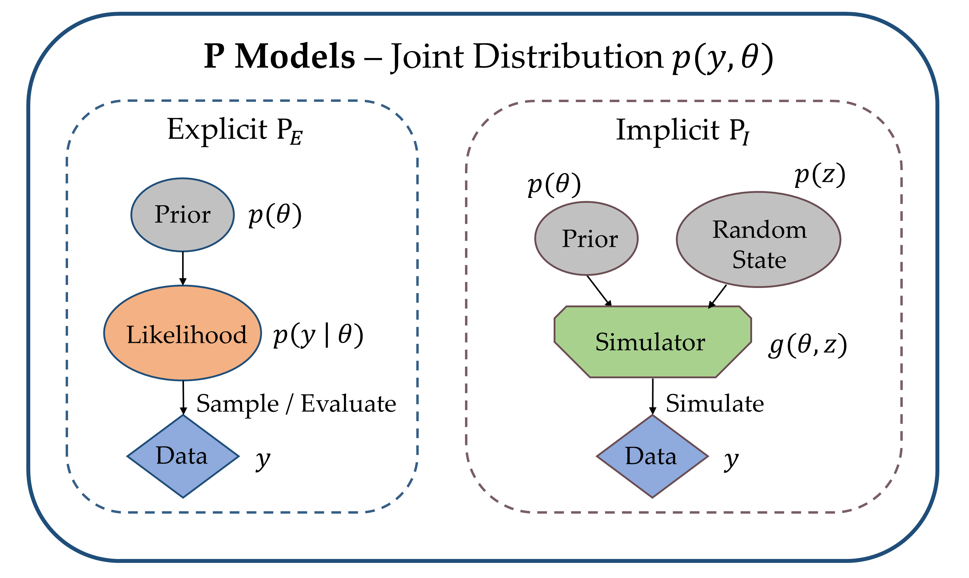
We can further draw a distinction between explicit likelihood P models and implicit likelihood P models (see Fig. 1).

Explicit Likelihood Models, abbreviated as $\textrm{P}_E$, are characterized by a tractable likelihood function. This means that the likelihood $p(y \, | \, \theta )$ is known analytically and its value can be evaluated for any pair $(y, \theta)$. $\textrm{P}_E$ models include popular statistical models, such as (generalized) linear and additive models [2], but also standard feedforward neural networks [1].

A simple example for an $\textrm{P}_E$ model is the canonical linear regression model, whose Bayesian recipe for $N$ pairs $(x_n, y_n)$ of vector-valued predictors $x_n \in \mathbb{R}^D$ and scalar outcomes $y_n \in \mathbb{R}$ can be written as

$$ \begin{align}
\theta &\sim \text{Normal}(0, \sigma_{\theta}^2 \cdot \mathbb{I}) \\
y_n &\sim \text{Normal}(\theta_0 + x_n^T\theta, \sigma_y) \quad \text{for} \quad n = 1,\dots,N.
\end{align} $$

Here, the symbol “$\sim$” means “distributed as”, $\sigma_y$ denotes the observation noise, and $\theta$ are the regression weights for which we have defined a multivariate Gaussian prior distribution with a spherical covariance $\sigma_{\theta}^2\cdot \mathbb{I}$. Importantly, everything in this P model is explicitly defined in terms of probability distributions and the likelihood is simply a Gaussian distribution whose density we can directly compute.

Implicit Likelihood Models, abbreviated as $\textrm{P}_I$, are defined by a Monte Carlo simulation program $y = g(\theta, z)$ and a prior $p(\theta)$, rather than directly through a likelihood function $p(y \, | \, \theta )$. The simulator $g$ transforms its inputs $\theta$ into outputs $y$ through a series of random program states $z$. Random program states can be any source of randomness in a simulation, which ensures that a single parameter configuration can lead to a variety of synthetic observations (in contrast to a deterministic mapping). Thus, a Monte Carlo simulator only implicitly defines the likelihood density via the relation

$$ p(y \, | \, \theta ) = \int_{\mathcal{Z}} p(y, z \mid \theta)\, \mathrm{d} z, $$

where $p(y, z \mid \theta)$ is the joint distribution of observables $y$ and random program states $z \in \mathcal{Z}$, if such a distribution over the (constrained) manifold $(y, z)$ exists. The above integral runs over all possible execution paths of the simulation program for a given input $\theta$ and is typically intractable, that is, we cannot explicitly write down the mathematical form of the implied likelihood $p(y \, | \, \theta )$.

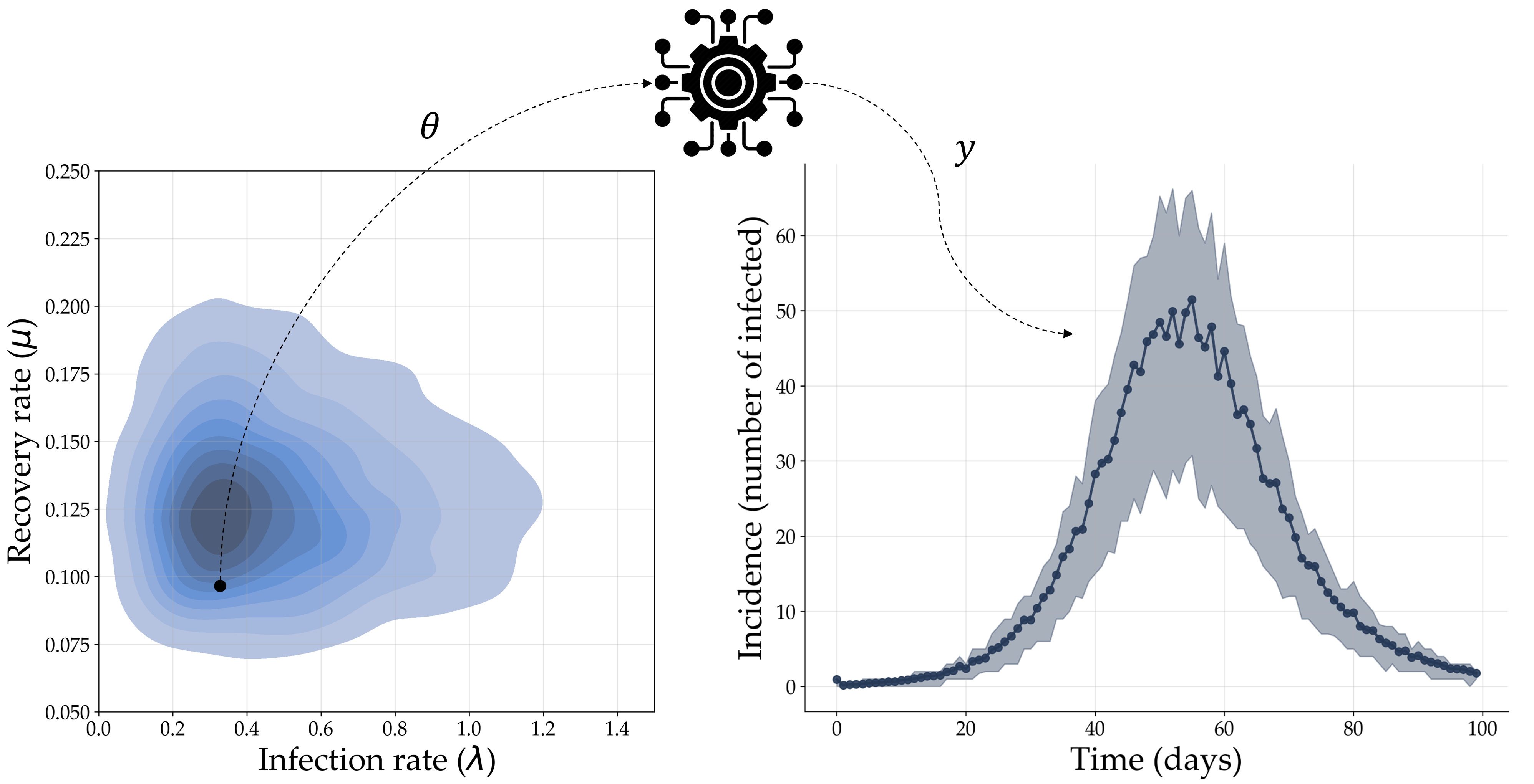
As an example, consider a simple model which describes the interaction dynamics between susceptible, $S$, infected, $I$, and recovered, $R$, individuals during a pandemic, with infection and recovery occurring at a constant transmission rate $\lambda$ and recovery rate $\mu$.

Suppose we are given a simulator which produces a discrete trajectory of incidence values (i.e., new infected cases) $y \equiv I_{new}$ for each parameter configuration $\theta = (\mu, \lambda)$. However, suppose that the simulator also injects noise into $y$ through an unknown random corruption process, thereby making the relationship between $\theta$ and $y$ non-deterministic. Since we do not have direct access to the corruption process, we cannot evaluate the likelihood $p(y \, | \, \theta )$ explicitly (as was the case for $\textrm{P}_E$ models). However, we can still analyze the probabilistic behavior of the model by running the simulator with different configurations $\theta$ drawn from a suitable prior $p(\theta)$. This process is depicted in Fig. 2.

Despite their apparent structural differences, $\textrm{P}_E$ and $\textrm{P}_I$ models can be analyzed with the same probabilistic toolkit. This speaks for the “unreasonable effectiveness” of Bayesian inference! For instance, we can define a formal notion of parsimony for an arbitrary P model by only using the consequences of probability theory.

P models and Occam’s Razor

Parsimony (i.e., the opposite of complexity) refers to the formal simplicity of a Bayesian model. We may also identify parsimony with the conceptual or mathematical elegance of the underlying interpretative framework, but this notion is less tractable. Curiously, each P model tacitly encodes a quantifiable notion of parsimony through its marginal likelihood (sometimes called Bayesian evidence, [3,4]). In principle, we can obtain the marginal likelihood of a P model by marginalizing the joint distribution $p(y, \theta)$ over its prior

$$ p(y) = \mathbb{E}_{p(\theta)}\left[p(y \, | \, \theta )\right] = \int_{\Theta} p(y \, | \, \theta )\, p(\theta) \, \mathrm d\theta, $$

where $\mathbb{E}_p$ denotes an expected value with respect to a reference distribution $p$ and we have left the dependence on the particular P model, which we would have expressed as $p(y \,|\, \textrm{P})$, implicit. We can interpret the marginal likelihood as the expected probability of generating data $y$ from a P model when we randomly sample from the prior $p(\theta)$. Through the prior’s role as a weight on the likelihood, the marginal likelihood encodes a probabilistic version of Occam’s razor by penalizing the prior complexity of a P model. Thus, we can use the marginal likelihood to compare competing P models based on an inherent trade-off between parsimony and the ability to fit the data.

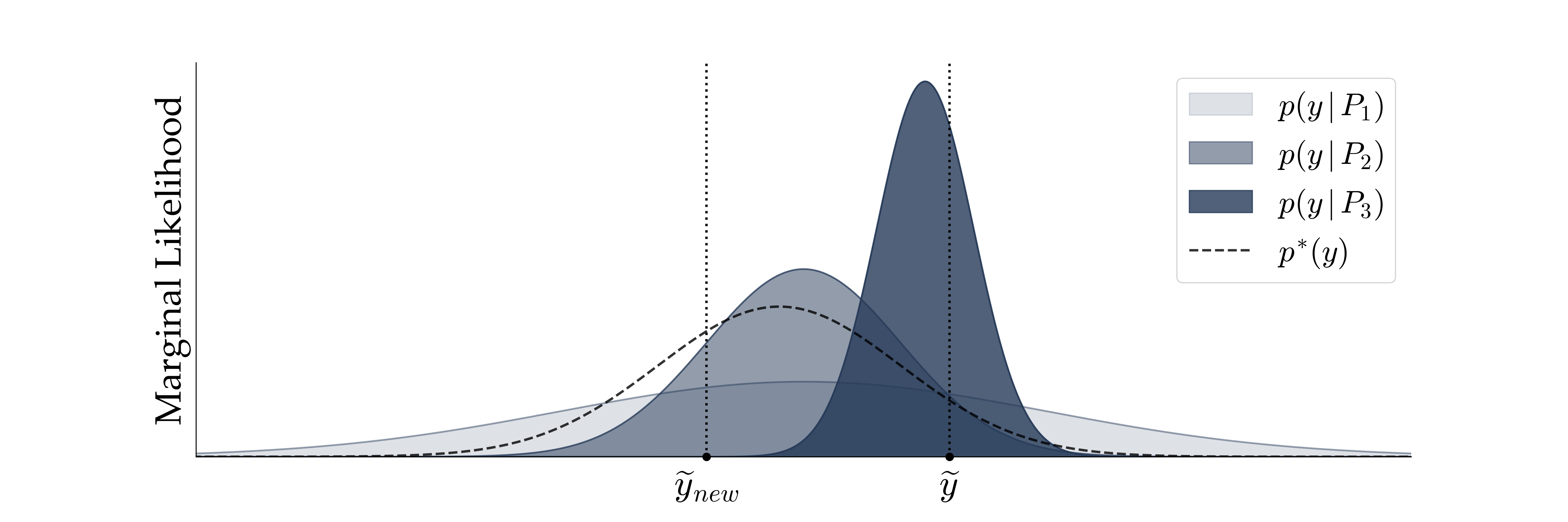
Fig. 3 illustrates a hypothetical model comparison scenario with three models of descending complexity: $\text{P}_1,$ $\text{P}_2,$ $\text{P}_3$. The most complex model $\text{P}_1$ can account for the broadest range of observations $y$ at the cost of diminished sharpness of its marginal likelihood, which is a straightforward consequence of probability theory (i.e., density functions should integrate to $1$). In contrast, the simplest model $\text{P}_3$ has the sharpest marginal likelihood which concentrates onto a narrow range of possible observations.

However, the marginal likelihood is a poor proxy for estimating the predictive performance, that is, how well a model can generalize beyond the data used for fitting. Consider two scalar observations $\tilde{y}$ and $\tilde{y}_{\text{new}}$, where we use the tilde to differentiate them from simulated observations. Even though $\tilde{y}$ is well within the generative scopes of models $\text{P}_1$ and $\text{P}_2$ too, the simplest model $\text{P}_3$ has the highest marginal likelihood at $\tilde{y}$ among the three candidates and is therefore favored from a marginal likelihood perspective. However, the higher relative marginal likelihood of the simplest model $\text{P}_3$ will assign close to zero density to the new (future) observation $\tilde{y}_{\text{new}}$, so, in a sense, the simplest model has overfit the data. The model $\text{P}_2$, whose marginal likelihood is closest to the data-generating distribution $p^{*}$, would have been favored, had $\tilde{y}_{\text{new}}$ instead of $\tilde{y}$ been used as the basis for model comparison.

In summary, we discussed the two main types of P models, namely those with explicit likelihoods (i.e., defined directly through a density function) and those with implicit likelihoods (i.e., defined through a randomized simulation program). In the next blog post, we will look at how to use P models for analyzing real data and the role of neural networks for modern Bayesian inference.

References

1. Ian Goodfellow, Yoshua Bengio, and Aaron Courville. Deep learning. MIT press, 2016.
2. Trevor Hastie, Robert Tibshirani, Jerome H Friedman, and Jerome H Friedman. The elements of statistical learning: data mining, inference, and prediction, volume 2. Springer, 2009.
3. Robert E Kass and Adrian E Raftery. Bayes factors. Journal of the american statistical association, 90(430):773–795, 1995.
4. David MacKay. Information theory, inference and learning algorithms. Cambridge University Press, 2003.