Predicting the Future: From Cave Paintings to DynaMix

Since the dawn of humanity, our ancestors have tried to predict the future by studying patterns in time. What began with Ice Age hunter-gatherers etching lunar cycles onto mammoth tusks has evolved into sophisticated algorithms that can forecast everything from the next financial market crash to disease surges weeks before hospitals feel the strain.

Today’s time series forecasting, the prediction of how systems like weather or ecosystems evolve in time, represents humanity’s most successful attempt yet to peer beyond the present. And it’s reshaping science, business, and society in ways we’re only beginning to understand.

The Rise of Time Series Foundation Models

The ancient quest to foresee the future has recently entered a new chapter with the emergence of time series foundation models (TSFM). These general-purpose AI systems learn by observing massive amounts of time-dependent data from all kinds of different application contexts. Just as large language models (LLMs), such as ChatGPT, revolutionized how machines read and generate text, TSFM are transforming how machines model and anticipate patterns that unfold over time. These patterns can originate from almost anywhere: climate measurements, traffic flow, brain activity, or financial markets – essentially, any process that changes over time.

Following the success of LLMs, researchers have developed powerful forecasting systems like Chronos, TimesFM or TimeGPT – models that can perform what scientists call zero-shot predictions: just from a given short time series snippet – and without any task-specific retraining – they are able to forecast how a new, unseen time series is likely to continue. These properties are what makes them so-called foundation models: once pretrained on broad datasets, they can perform many different forecasting tasks without having to be retrained from scratch for each one. In this way, a single model is capable of making meaningful predictions for the future evolution of a vast array of natural or engineered systems – not because it “knows” the underlying laws or principles, but because it has come across a sufficient number of examples to recognize recurrent patterns in data from various different contexts.

At their core, most TSFM are built on the same kind of neural architecture – the transformer – that powers large language models like GPT and Llama. Originally drawing on analogies to the brain, neural architectures consist of networks of many small computational units (or “neurons”) that manipulate signals by performing simple calculations. Working together, a large number of such artificial neurons can uncover remarkably complex patterns. TSFM adapt this architecture from natural language to time-based data: they treat short snippets from time series similar to sequences of “words” – so-called tokens. However, there is a catch.

Pattern Matching Isn’t Understanding

For all their sophistication, current foundation models operate primarily as pattern-matching devices. This means they are very successful at learning statistical regularities – without being aware of the dynamical rules that actually generate the behaviour we observe. As a result, they are very good at predicting the next few steps in a sequence, but often struggle with long-term predictions. Their forecasts may quickly drift away from the true behaviour, especially when the underlying mechanisms are complex or chaotic, as is the case for weather patterns or brain activity.

An effective way to overcome this limitation is by shifting from simply learning patterns in the data to learning the structure of the process that produces that data. This is the idea behind DynaMix, a new AI model developed in our working group. DynaMix is the first foundation model that doesn’t just forecast the future, but recovers the mathematical structure underlying the observed phenomena. In particular, DynaMix learns the structure of what’s called the dynamical system underlying the data.

The study of dynamical systems is quite old. It has ancient roots in humanity’s earliest attempts to model the motions of the Sun, Moon, and planets. The field took on a more formal shape in the 17th century, when scientists like Isaac Newton began writing down mathematical laws that described how the motion of physical bodies in space evolves step by step. Over centuries, this grew into a rich branch of science and mathematics concerned with the rules that govern any system that changes over time. Dynamical systems theory has introduced universal concepts for describing how a variety of time-dependent processes unfold in nature – be it the weather shifting from day to day, cars moving through streets, or neurons firing in the brain.

At the heart of dynamical systems theory lies the idea that time-dependent systems “move” through a state space – an abstract space encompassing all conditions the system can possibly be found in. As the system evolves, it traces out a path through this space, and over sufficiently long periods its path may form clear geometric patterns. As an example, many systems are drawn toward particular regions or shapes in state space, known as attractors. An attractor is a geometrical object into which trajectories are ultimately pulled. They can be thought of as sets of possible states a system might be in the future. For instance, in the brain this might be the set of all firing rates the neurons might assume. Locating attractors in state space can reveal what kinds of behaviour might be typical for a system and which states it will almost never visit.

Learning Dynamical Systems With AI

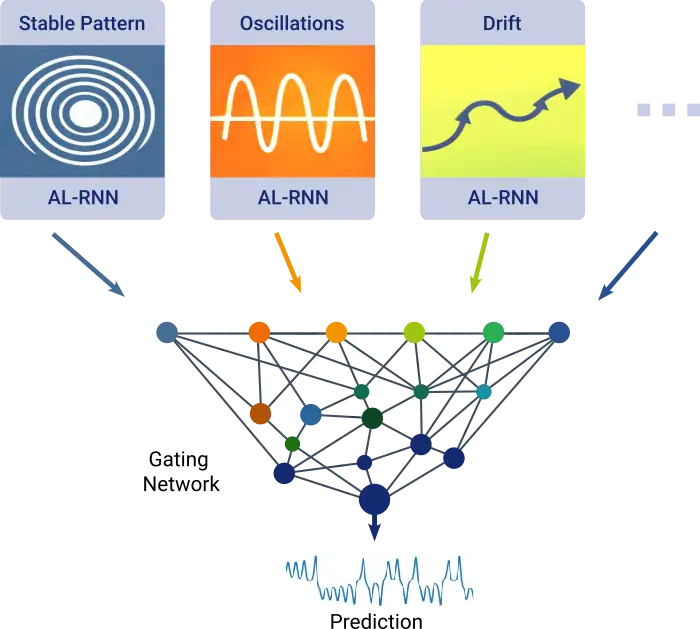
In order to be able to capture the structure of attractors and other features of dynamical systems, DynaMix must be able to represent many different kinds of behaviours typical for dynamical systems – from stable patterns to oscillations, drifts or chaotic evolution. This is why DynaMix employs a so-called mixture-of-experts framework: instead of relying on one large model that tries to handle everything at once, many small forecasting modules (so-called AL-RNNs, for Almost Linear Recurrent Neural Networks) each learn a particular style of dynamical behaviour and cast their vote on what the future might look like. In the end, a so-called gating network combines all these votes into a single coherent prediction.

This enables DynaMix to achieve accurate long-term predictions. In contrast to other current foundation models, it is able to predict the geometry of trajectories – the way in which all variables describing the system (like temperatures or biological species) jointly change within the space of possible states. In complex or even chaotic systems, where future evolution is extremely sensitive to initial conditions, this does not mean predicting one exact future path. Rather, it means capturing the characteristic long-range patterns, shapes, and statistical regularities that define the system’s behaviour over time.

Chaotic systems

Chaotic systems are notoriously hard to learn from data because tiny errors in prediction can grow rapidly. In order to be able to make well-informed forecasts nonetheless, DynaMix uses special training algorithms, called sparse and generalized teacher forcing. These techniques come from control theory – a branch of engineering and mathematics that studies how to guide systems so they behave in stable, predictable ways. These techniques prevent the model’s training from drifting or exploding, allowing it to learn stable, meaningful long-term behaviour from data that would otherwise be difficult to handle. For DynaMix they also enable it to learn stable representations of complex dynamics without the massive parameter load required by transformer-based foundation models.

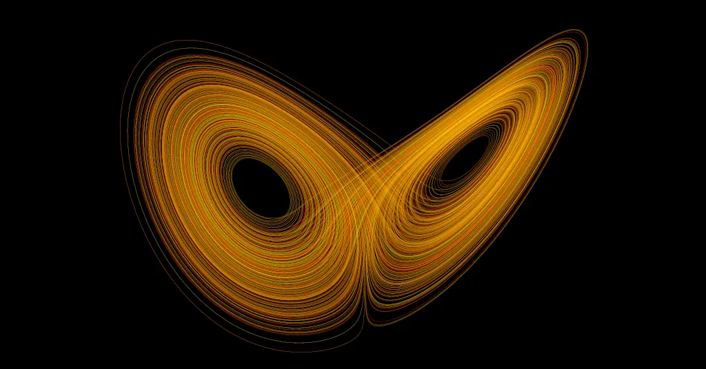
An example of a system that is both chaotic and an attractor is the Lorenz attractor, a dynamical system originally formulated as a model for atmospheric convection. Even though the Lorenz attractor is governed by deterministic rules, its motion is inherently chaotic: trajectories that start nearly identically diverge quickly. At the same time, all trajectories are drawn toward a characteristic “butterfly-shaped” region (see Fig. 2 below). Thus, regardless of initial conditions, the long-term evolution remains confined to the same region – without ever repeating exactly.

How Well Does DynaMix Work?

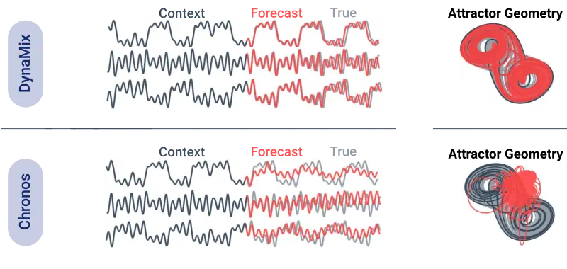
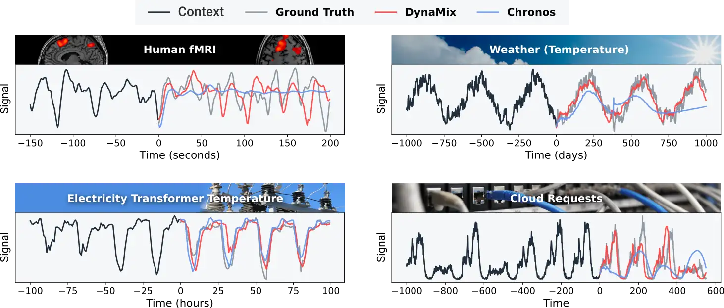
DynaMix’s capability to predict the geometry of trajectories enables it to perform both short- and long-term predictions on novel systems after being trained exclusively on a small but diverse corpus of only 34 simulated dynamical systems. This is demonstrated in Fig. 3, where DynaMix was provided with a short time series snippet, the “context”, from a previously unseen dynamical system whose temporal evolution it had to forecast into the long future. Its performance here is compared to Chronos, an existing AI model. As can be seen, DynaMix outperforms current time series foundation models not only with regard to long-term forecasts. In this example, and many more cases, it surpasses them in short-term prediction as well. That DynaMix achieves this with its rather small training corpus challenges conventional wisdom, which posits that massive training datasets are required for such a generalization to occur – a surprising result.

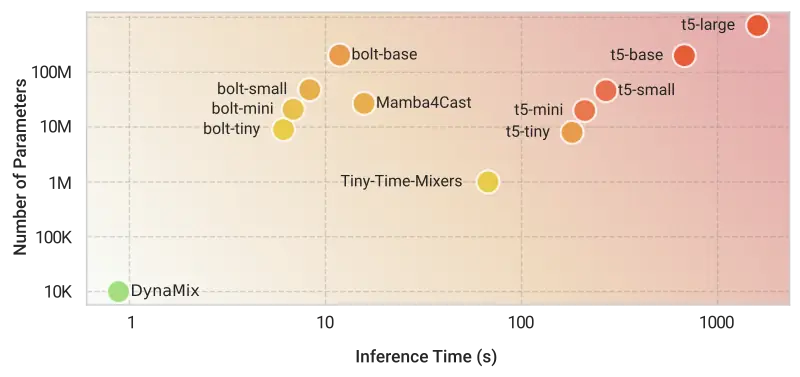
Remarkably, DynaMix surpasses TSFMs in performance while at the same time requiring far fewer computational resources. Most transformer-based time series models contain hundreds of millions, sometimes billions of parameters – making them computationally expensive. DynaMix, in contrast, uses only a tiny fraction of those parameters, and thus also produces forecasts orders of magnitude faster, as can be seen in Fig. 4. This efficiency matters because it expands what is possible: forecasts can now be carried out at scale where other models may be far too slow or expensive.

Aside from accuracy and efficiency, there are fundamental new things we are able to learn from applying DynaMix to real-world data. Due to its design based on AL-RNNs, the model also offers a degree of insight into dynamical systems that other foundation models lack. In particular, this makes it possible to understand which aspects of a system drive predicted future behaviour – offering researchers interpretable insights into the underlying mechanisms rather than merely black-box predictions.

The Road Ahead

Seen in a wider context, combining zero-shot inference capabilities with rigorous dynamical systems reconstruction marks a fundamental shift in time series modeling and forecasting. DynaMix, the AI model that we have developed within the STRUCTURES cluster, pioneers a new approach to temporal analysis that moves beyond pattern recognition to actual mechanism recovery. By linking modern AI to the mathematics of dynamical systems, the approach blurs the boundary between prediction and explanation.

This shift opens new possibilities for both scientific discovery and time series prediction, enabling us to look beyond the hood and understand the structural dynamical principles governing time series evolution. In the future, such AI models may help us understand not just what will happen, but why.

Try it out – DynaMix on HuggingFace: https://huggingface.co/spaces/DurstewitzLab/DynaMix

Scientific Reference

Christoph Hemmer & Daniel Durstewitz, True Zero-Shot Inference of Dynamical Systems Preserving Long-Term Statistics, 2025, Advances in Neural Information Processing Systems, https://arxiv.org/abs/2505.13192